pyxu.operator.linop#
Basic Operators#
- class SubSample(dim_shape, *indices)[source]#
Bases:
LinOpMulti-dimensional sub-sampling operator.
This operator extracts a subset of the input matching the provided subset specifier. Its Lipschitz constant is 1.
Examples
### Extract even samples of a 1D signal.
import pyxu.operator as pxo
x = np.arange(10)
S = pxo.SubSample(
      x.shape,
      slice(0, None, 2),
)
y = S(x)  # array([0, 2, 4, 6, 8])
### Extract columns[1, 3, -1] from a 2D matrix
import pyxu.operator as pxo
x = np.arange(3 * 40).reshape(3, 40)  # the input
S = pxo.SubSample(
      x.shape,
      slice(None),  # take all rows
      [1, 3, -1],   # and these columns
)
y = S(x)  # array([[  1.,   3.,  39.],
          #        [ 41.,  43.,  79.],
          #        [ 81.,  83., 119.]])
### Extract all red rows of an (D,H,W) RGB image matching a boolean mask.
import pyxu.operator as pxo
x = np.arange(3 * 5 * 4).reshape(3, 5, 4)
mask = np.r_[True, False, False, True, False]
S = pxo.SubSample(
      x.shape,
      0,            # red channel
      mask,         # row selector
      slice(None),  # all columns; this field can be omitted.
)
y = S(x)  # array([[[ 0,  1,  2,  3],
          #         [12, 13, 14, 15]]])
- Parameters:
- __init__(dim_shape, *indices)[source]#
- Parameters:
dim_shape (
NDArrayShape) – (M1,…,MD) domain dimensions.indices (
IndexSpec) –Sub-sample specifier per dimension. (See examples.)
Valid specifiers are:
integers
1D sequence of int/bool-s
slices
Unspecified trailing dimensions are not sub-sampled.
Notes
The co-dimension rank always matches the dimension rank, i.e. sub-sampling does not drop dimensions. Single-element dimensions can be removed by composing
SubSamplewithSqueezeAxes.
- Trim(dim_shape, trim_width)[source]#
Multi-dimensional trimming operator.
This operator trims the input array in each dimension according to specified widths.
- Parameters:
dim_shape (
NDArrayShape) – (M1,…,MD) domain dimensions.trim_width (
TrimSpec) –Number of values trimmed from the edges of each axis. Multiple forms are accepted:
int: trim each dimension’s head/tail bytrim_width.tuple[int, ...]: trim dimension[k]’s head/tail bytrim_width[k].tuple[tuple[int, int], ...]: trim dimension[k]’s head/tail bytrim_width[k][0]/trim_width[k][1]respectively.
- Returns:
op
- Return type:
- class Sum(dim_shape, axis=None)[source]#
Bases:
LinOpMulti-dimensional sum reduction \(\mathbf{A}: \mathbb{R}^{M_{1} \times\cdots\times M_{D}} \to \mathbb{R}^{N_{1} \times\cdots\times N_{D}}\).
Notes
The co-dimension rank always matches the dimension rank, i.e. summed-over dimensions are not dropped. Single-element dimensions can be removed by composing
SumwithSqueezeAxes.The matrix operator of a 1D reduction applied to \(\mathbf{x} \in \mathbb{R}^{M}\) is given by
\[\mathbf{A}(x) = \mathbf{1}^{T} \mathbf{x},\]where \(\sigma_{\max}(\mathbf{A}) = \sqrt{M}\). An ND reduction is a chain of 1D reductions in orthogonal dimensions. Hence the Lipschitz constant of an ND reduction is the product of Lipschitz constants of all 1D reductions involved, i.e.:
\[L = \sqrt{\prod_{i_{k}} M_{i_{k}}},\]where \(\{i_{k}\}_{k}\) denotes the axes being summed over.
- __init__(dim_shape, axis=None)[source]#
Multi-dimensional sum reduction.
- Parameters:
dim_shape (
NDArrayShape) – (M1,…,MD) domain dimensions.axis (
NDArrayAxis) – Axis or axes along which a sum is performed. The default, axis=None, will sum all the elements of the input array.
- adjoint(arr)[source]#
Evaluate operator adjoint at specified point(s).
- Parameters:
arr (
NDArray) – (…, N1,…,NK) input points.- Returns:
out – (…, M1,…,MD) adjoint evaluations.
- Return type:
Notes
The adjoint \(\mathbf{A}^{\ast}: \mathbb{R}^{N_{1} \times\cdots\times N_{K}} \to \mathbb{R}^{M_{1} \times\cdots\times M_{D}}\) of \(\mathbf{A}: \mathbb{R}^{M_{1} \times\cdots\times M_{D}} \to \mathbb{R}^{N_{1} \times\cdots\times N_{K}}\) is defined as:
\[\langle \mathbf{x}, \mathbf{A}^{\ast}\mathbf{y}\rangle_{\mathbb{R}^{M_{1} \times\cdots\times M_{D}}} := \langle \mathbf{A}\mathbf{x}, \mathbf{y}\rangle_{\mathbb{R}^{N_{1} \times\cdots\times N_{K}}}, \qquad \forall (\mathbf{x},\mathbf{y})\in \mathbb{R}^{M_{1} \times\cdots\times M_{D}} \times \mathbb{R}^{N_{1} \times\cdots\times N_{K}}.\]
- estimate_lipschitz(**kwargs)[source]#
Compute a Lipschitz constant of the operator.
- Parameters:
- Return type:
Notes
The tightest Lipschitz constant is given by the spectral norm of the operator \(\mathbf{A}\): \(\|\mathbf{A}\|_{2}\). It can be computed via the SVD, which is compute-intensive task for large operators. In this setting, it may be advantageous to overestimate the Lipschitz constant with the Frobenius norm of \(\mathbf{A}\) since \(\|\mathbf{A}\|_{F} \geq \|\mathbf{A}\|_{2}\).
\(\|\mathbf{A}\|_{F}\) can be efficiently approximated by computing the trace of \(\mathbf{A}^{\ast} \mathbf{A}\) (or \(\mathbf{A}\mathbf{A}^{\ast}\)) via the Hutch++ stochastic algorithm.
\(\|\mathbf{A}\|_{F}\) is upper-bounded by \(\|\mathbf{A}\|_{F} \leq \sqrt{n} \|\mathbf{A}\|_{2}\), where the equality is reached (worst-case scenario) when the eigenspectrum of the linear operator is flat.
- class IdentityOp(dim_shape)[source]#
Bases:
OrthProjOpIdentity operator.
- class NullOp(dim_shape, codim_shape)[source]#
Bases:
LinOpNull operator.
This operator maps any input vector on the null vector.
- NullFunc(dim_shape)[source]#
Null functional.
This functional maps any input vector on the null scalar.
- HomothetyOp(dim_shape, cst)[source]#
Constant scaling operator.
- Parameters:
- Returns:
op – Scaling operator.
- Return type:
Note
This operator is not defined in terms of
DiagonalOp()since it is array-backend-agnostic.
- DiagonalOp(vec, dim_shape=None, enable_warnings=True)[source]#
Element-wise scaling operator.
Note
DiagonalOp()instances are not arraymodule-agnostic: they will only work with NDArrays belonging to the same array module asvec. Moreover, inner computations may cast input arrays when the precision ofvecdoes not match the user-requested precision. If such a situation occurs, a warning is raised.If
vecis a DASK array, the operator will be aSelfAdjointOp. Ifvecis a NUMPY/CUPY array, the created operator specializes toPosDefOpwhen possible. Specialization is not automatic for DASK inputs because operators should be quick to build under all circumstances, and this is not guaranteed if we have to check that all entries are positive for out-of-core arrays. Users who know that allvecentries are positive can manually cast toPosDefOpafterwards if required.
- Parameters:
dim_shape (
NDArrayShape) – (M1,…,MD) shape of operator’s domain. Defaults to the shape ofvecwhen omitted.vec (
NDArray) – Scale factors. Ifdim_shapeis provided, thenvecmust be broadcastable with arrays of sizedim_shape.enable_warnings (
bool) – IfTrue, emit a warning in case of precision mis-match issues.
- Return type:
- class Pad(dim_shape, pad_width, mode='constant')[source]#
Bases:
LinOpMulti-dimensional padding operator.
This operator pads the input array in each dimension according to specified widths.
Notes
If inputs are D-dimensional, then some of the padding of later axes are calculated from padding of previous axes.
The adjoint of the padding operator performs a cumulative summation over the original positions used to pad. Its effect is clear from its matrix form. For example the matrix-form of
Pad(dim_shape=(3,), mode="wrap", pad_width=(1, 1))is:\[\begin{split}\mathbf{A} = \left[ \begin{array}{ccc} 0 & 0 & 1 \\ 1 & 0 & 0 \\ 0 & 1 & 0 \\ 0 & 0 & 1 \\ 1 & 0 & 0 \end{array} \right].\end{split}\]The adjoint of \(\mathbf{A}\) corresponds to its matrix transpose:
\[\begin{split}\mathbf{A}^{\ast} = \left[ \begin{array}{ccccc} 0 & 1 & 0 & 0 & 1 \\ 0 & 0 & 1 & 0 & 0 \\ 1 & 0 & 0 & 1 & 0 \end{array} \right].\end{split}\]This operation can be seen as a trimming (\(\mathbf{T}\)) plus a cumulative summation (\(\mathbf{S}\)):
\[\begin{split}\mathbf{A}^{\ast} = \mathbf{T} + \mathbf{S} = \left[ \begin{array}{ccccc} 0 & 1 & 0 & 0 & 0 \\ 0 & 0 & 1 & 0 & 0 \\ 0 & 0 & 0 & 1 & 0 \end{array} \right] + \left[ \begin{array}{ccccc} 0 & 0 & 0 & 0 & 1 \\ 0 & 0 & 0 & 0 & 0 \\ 1 & 0 & 0 & 0 & 0 \end{array} \right],\end{split}\]where both \(\mathbf{T}\) and \(\mathbf{S}\) are efficiently implemented in matrix-free form.
The Lipschitz constant of the multi-dimensional padding operator is upper-bounded by the product of Lipschitz constants of the uni-dimensional paddings applied per dimension, i.e.:
\[L \le \prod_{i} L_{i}, \qquad i \in \{1, \ldots, D\},\]where \(L_{i}\) depends on the boundary condition at the \(i\)-th axis.
\(L_{i}^{2}\) corresponds to the maximum singular value of the diagonal matrix
\[\mathbf{A}_{i}^{\ast} \mathbf{A}_{i} = \mathbf{T}_{i}^{\ast} \mathbf{T}_{i} + \mathbf{S}_{i}^{\ast} \mathbf{S}_{i} = \mathbf{I}_{N} + \mathbf{S}_{i}^{\ast} \mathbf{S}_{i}.\]In mode=”constant”, \(\text{diag}(\mathbf{S}_{i}^{\ast} \mathbf{S}_{i}) = \mathbf{0}\), hence \(L_{i} = 1\).
In mode=”edge”,
\[\text{diag}(\mathbf{S}_{i}^{\ast} \mathbf{S}_{i}) = \left[p_{lhs}, 0, \ldots, 0, p_{rhs} \right],\]hence \(L_{i} = \sqrt{1 + \max(p_{lhs}, p_{rhs})}\).
In mode=”symmetric”, “wrap”, “reflect”, \(\text{diag}(\mathbf{S}_{i}^{\ast} \mathbf{S}_{i})\) equals (up to a mode-dependant permutation)
\[\text{diag}(\mathbf{S}_{i}^{\ast} \mathbf{S}_{i}) = \left[1, \ldots, 1, 0, \ldots, 0\right] + \left[0, \ldots, 0, 1, \ldots, 1\right],\]hence
\[\begin{split}L^{\text{wrap, symmetric}}_{i} = \sqrt{1 + \lceil\frac{p_{lhs} + p_{rhs}}{N}\rceil}, \\ L^{\text{reflect}}_{i} = \sqrt{1 + \lceil\frac{p_{lhs} + p_{rhs}}{N-2}\rceil}.\end{split}\]
- Parameters:
- __init__(dim_shape, pad_width, mode='constant')[source]#
- Parameters:
dim_shape (
NDArrayShape) – (M1,…,MD) domain dimensions.pad_width (
WidthSpec) –Number of values padded to the edges of each axis. Multiple forms are accepted:
int: pad each dimension’s head/tail bypad_width.tuple[int, ...]: pad dimension[k]’s head/tail bypad_width[k].tuple[tuple[int, int], ...]: pad dimension[k]’s head/tail bypad_width[k][0]/pad_width[k][1]respectively.
Padding mode. Multiple forms are accepted:
str: unique mode shared amongst dimensions. Must be one of:
’constant’ (zero-padding)
’wrap’
’reflect’
’symmetric’
’edge’
tuple[str, …]: pad dimension[k] using
mode[k].
(See
numpy.pad()for details.)
Transforms#
- class FFT(dim_shape, axes=None, **kwargs)[source]#
Bases:
NormalOpMulti-dimensional Discrete Fourier Transform (DFT) \(A: \mathbb{C}^{M_{1} \times\cdots\times M_{D}} \to \mathbb{C}^{M_{1} \times\cdots\times M_{D}}\).
The FFT is defined as follows:
\[(A \, \mathbf{x})[\mathbf{k}] = \sum_{\mathbf{n}} \mathbf{x}[\mathbf{n}] \exp\left[-j 2 \pi \langle \frac{\mathbf{n}}{\mathbf{N}}, \mathbf{k} \rangle \right],\]\[(A^{*} \, \hat{\mathbf{x}})[\mathbf{n}] = \sum_{\mathbf{k}} \hat{\mathbf{x}}[\mathbf{k}] \exp\left[j 2 \pi \langle \frac{\mathbf{n}}{\mathbf{N}}, \mathbf{k} \rangle \right],\]\[(\mathbf{x}, \, \hat{\mathbf{x}}) \in \mathbb{C}^{M_{1} \times\cdots\times M_{D}}, \quad (\mathbf{n}, \, \mathbf{k}) \in \{0, \ldots, M_{1}-1\} \times\cdots\times \{0, \ldots, M_{D}-1\}.\]The DFT is taken over any number of axes by means of the Fast Fourier Transform algorithm (FFT).
Implementation Notes
The CPU implementation uses SciPy’s FFT implementation.
The GPU implementation uses cuFFT via CuPy.
The DASK implementation evaluates the FFT in chunks using the CZT algorithm.
Caveat: the cost of assembling the DASK graph grows with the total number of chunks; just calling
FFT.apply()may take a few seconds or more if inputs are highly chunked. Performance is ~7-10x slower than equivalent non-chunked NUMPY version (assuming it fits in memory).
Examples
1D DFT of a cosine pulse.
from pyxu.operator import FFT
import pyxu.util as pxu

N = 10
op = FFT(N)

x = np.cos(2 * np.pi / N * np.arange(N), dtype=complex)  # (N,)
x_r = pxu.view_as_real(x)                                # (N, 2)

y_r = op.apply(x_r)                                      # (N, 2)
y = pxu.view_as_complex(y_r)                             # (N,)
# [0, N/2, 0, 0, 0, 0, 0, 0, 0, N/2]

z_r = op.adjoint(op.apply(x_r))                          # (N, 2)
z = pxu.view_as_complex(z_r)                             # (N,)
# np.allclose(z, N * x) -> True
1D DFT of a complex exponential pulse.
from pyxu.operator import FFT
import pyxu.util as pxu

N = 10
op = FFT(N)

x = np.exp(1j * 2 * np.pi / N * np.arange(N))            # (N,)
x_r = pxu.view_as_real(x)                                # (N, 2)

y_r = op.apply(x_r)                                      # (N, 2)
y = pxu.view_as_complex(y_r)                             # (N,)
# [0, N, 0, 0, 0, 0, 0, 0, 0, 0]

z_r = op.adjoint(op.apply(x_r))                          # (N, 2)
z = pxu.view_as_complex(z_r)                             # (N,)
# np.allclose(z, N * x) -> True
2D DFT of an image
from pyxu.operator import FFT
import pyxu.util as pxu

N_h, N_w = 10, 8
op = FFT((N_h, N_w))

x = np.pad(                                              # (N_h, N_w)
    np.ones((N_h//2, N_w//2), dtype=complex),
    pad_width=((0, N_h//2), (0, N_w//2)),
)
x_r = pxu.view_as_real(x)                                # (N_h, N_w, 2)

y_r = op.apply(x_r)                                      # (N_h, N_w, 2)
y = pxu.view_as_complex(y_r)                             # (N_h, N_w)

z_r = op.adjoint(op.apply(x_r))                          # (N_h, N_w, 2)
z = pxu.view_as_complex(z_r)                             # (N_h, N_w)
# np.allclose(z, (N_h * N_w) * x) -> True
- __init__(dim_shape, axes=None, **kwargs)[source]#
- Parameters:
dim_shape (
NDArrayShape) – (M1,…,MD) dimensions of the input \(\mathbf{x} \in \mathbb{C}^{M_{1} \times\cdots\times M_{D}}\).axes (
NDArrayAxis) – Axes over which to compute the FFT. If not given, all axes are used.kwargs (
dict) –Extra kwargs passed to
scipy.fft.fftn()orcupyx.scipy.fft.fftn().Supported parameters for
scipy.fft.fftn()are:workers: int = None
Supported parameters for
cupyx.scipy.fft.fftn()are:NOT SUPPORTED FOR NOW
Default values are chosen if unspecified.
- apply(arr)[source]#
- Parameters:
arr (
NDArray) – (…, M1,…,MD,2) inputs \(\mathbf{x} \in \mathbb{C}^{M_{1} \times\cdots\times M_{D}}\) viewed as a real array. (Seeview_as_real().)- Returns:
out – (…, M1,…,MD,2) outputs \(\hat{\mathbf{x}} \in \mathbb{C}^{M_{1} \times\cdots\times M_{D}}\) viewed as a real array. (See
view_as_real().)- Return type:
- adjoint(arr)[source]#
- Parameters:
arr (
NDArray) – (…, M1,…,MD,2) inputs \(\hat{\mathbf{x}} \in \mathbb{C}^{M_{1} \times\cdots\times M_{D}}\) viewed as a real array. (Seeview_as_real().)- Returns:
out – (…, M1,…,MD,2) outputs \(\mathbf{x} \in \mathbb{C}^{M_{1} \times\cdots\times M_{D}}\) viewed as a real array. (See
view_as_real().)- Return type:
- class CZT(dim_shape, axes, M, A, W, **kwargs)[source]#
Bases:
LinOpMulti-dimensional Chirp Z-Transform (CZT) \(C: \mathbb{C}^{N_{1} \times\cdots\times N_{D}} \to \mathbb{C}^{M_{1} \times\cdots\times M_{D}}\).
The 1D CZT of parameters \((A, W, M)\) is defined as:
\[(C \, \mathbf{x})[k] = \sum_{n=0}^{N-1} \mathbf{x}[n] A^{-n} W^{nk},\]where \(\mathbf{x} \in \mathbb{C}^{N}\), \(A, W \in \mathbb{C}\), and \(k = \{0, \ldots, M-1\}\).
A D-dimensional CZT corresponds to taking a 1D CZT along each transform axis.
Implementation Notes
For stability reasons, this implementation assumes \(A, W \in \mathbb{C}\) lie on the unit circle.
See also
- __init__(dim_shape, axes, M, A, W, **kwargs)[source]#
- Parameters:
dim_shape (
NDArrayShape) – (N1,…,ND) dimensions of the input \(\mathbf{x} \in \mathbb{C}^{N_{1} \times\cdots\times N_{D}}\).axes (
NDArrayAxis) – Axes over which to compute the CZT. If not given, all axes are used.M (
int,list(int)) – Length of the transform per axis.A (
complex,list(complex)) – Circular offset from the positive real-axis per axis.W (
complex,list(complex)) – Circular spacing between transform points per axis.
- apply(arr)[source]#
- Parameters:
arr (
NDArray) – (…, N1,…,ND,2) inputs \(\mathbf{x} \in \mathbb{C}^{N_{1} \times\cdots\times N_{D}}\) viewed as a real array. (Seeview_as_real().)- Returns:
out – (…, M1,…,MD,2) outputs \(\hat{\mathbf{x}} \in \mathbb{C}^{M_{1} \times\cdots\times M_{D}}\) viewed as a real array. (See
view_as_real().)- Return type:
- adjoint(arr)[source]#
- Parameters:
arr (
NDArray) – (…, M1,…,MD,2) inputs \(\hat{\mathbf{x}} \in \mathbb{C}^{M_{1} \times\cdots\times M_{D}}\) viewed as a real array. (Seeview_as_real().)- Returns:
out – (…, N1,…,ND,2) outputs \(\mathbf{x} \in \mathbb{C}^{N_{1} \times\cdots\times N_{D}}\) viewed as a real array. (See
view_as_real().)- Return type:
Stencils & Convolutions#
- class _Stencil(kernel, center)[source]#
Bases:
objectMulti-dimensional JIT-compiled stencil. (Low-level function.)
This low-level class creates a gu-vectorized stencil applicable on multiple inputs simultaneously. Only NUMPY/CUPY arrays are accepted.
Create instances via factory method
init().Example
Correlate a stack of images
Awith a (3, 3) kernel such that:\[B[n, m] = A[n-1, m] + A[n, m-1] + A[n, m+1] + A[n+1, m]\]import numpy as np from pyxu.operator import _Stencil # create the stencil kernel = np.array([[0, 1, 0], [1, 0, 1], [0, 1, 0]], dtype=np.float64) center = (1, 1) stencil = _Stencil.init(kernel, center) # apply it to the data rng = np.random.default_rng() A = rng.normal(size=(2, 3, 4, 30, 30)) # 24 images of size (30, 30) B = np.zeros_like(A) stencil.apply(A, B) # (2, 3, 4, 30, 30)
- apply(arr, out, **kwargs)[source]#
Evaluate stencil on multiple inputs.
- Parameters:
arr (
NDArray) – (…, M1,…,MD) data to process.out (
NDArray) – (…, M1,…,MD) array to which outputs are written.kwargs (
dict) –Extra kwargs to configure
f_jit(), the Dispatcher instance created by Numba.Only relevant for GPU stencils, with values:
blockspergrid: int
threadsperblock: int
Default values are chosen if unspecified.
- Returns:
out – (…, M1,…,MD) outputs.
- Return type:
Notes
arrandoutmust have the same type/dtype as the kernel used during instantiation.Index regions in
outwhere the stencil is not fully supported are set to 0.apply()may raiseCUDA_ERROR_LAUNCH_OUT_OF_RESOURCESwhen the number of GPU registers required exceeds resource limits. There are 2 solutions to this problem:Pass the
max_registerskwarg to f_jit()’s decorator; or
must be set at compile time; it is thus left unbounded.
is accessible through .apply(**kwargs).
- class Stencil(dim_shape, kernel, center, mode='constant', enable_warnings=True)[source]#
Bases:
SquareOpMulti-dimensional JIT-compiled stencil.
Stencils are a common computational pattern in which array elements are updated according to some fixed pattern called the stencil kernel. Notable examples include multi-dimensional convolutions, correlations and finite differences. (See Notes for a definition.)
Stencils can be evaluated efficiently on CPU/GPU architectures.
Several boundary conditions are supported. Moreover boundary conditions may differ per axis.
Implementation Notes
Numba (and its
@stencildecorator) is used to compile efficient machine code from a stencil kernel specification. This has 2 consequences:Stencilinstances are not arraymodule-agnostic: they will only work with NDArraysbelonging to the same array module as
kernel.
Compiled stencils are not precision-agnostic: they will only work on NDArrays with the same dtype as
kernel. A warning is emitted if inputs must be cast to the kernel dtype.
Stencil kernels can be specified in two forms: (See
__init__()for details.)A single non-separable \(D\)-dimensional kernel \(k[i_{1},\ldots,i_{D}]\) of shape \((K_{1},\ldots,K_{D})\).
A sequence of separable \(1\)-dimensional kernel(s) \(k_{d}[i]\) of shapes \((K_{1},),\ldots,(K_{D},)\) such that \(k[i_{1},\ldots,i_{D}] = \Pi_{d=1}^{D} k_{d}[i_{d}]\).
Mathematical Notes
Given a \(D\)-dimensional array \(x\in\mathbb{R}^{N_1\times\cdots\times N_D}\) and kernel \(k\in\mathbb{R}^{K_1\times\cdots\times K_D}\) with center \((c_1, \ldots, c_D)\), the output of the stencil operator is an array \(y\in\mathbb{R}^{N_1\times\cdots\times N_D}\) given by:
\[y[i_{1},\ldots,i_{D}] = \sum_{q_{1},\ldots,q_{D}=0}^{K_{1},\ldots,K_{D}} x[i_{1} - c_{1} + q_{1},\ldots,i_{D} - c_{D} + q_{D}] \,\cdot\, k[q_{1},\ldots,q_{D}].\]This corresponds to a correlation with a shifted version of the kernel \(k\).
Numba stencils assume summation terms involving out-of-bound indices of \(x\) are set to zero.
Stencillifts this constraint by extending the stencil to boundary values via pre-padding and post-trimming. Concretely, any stencil operator \(S\) instantiated withStencilcan be written as the composition \(S = TS_0P\), where \((T, S_0, P)\) are trimming, stencil with zero-padding conditions, and padding operators respectively. This construct allowsStencilto handle complex boundary conditions under which \(S\) may not be a proper stencil (i.e., varying kernel) but can still be implemented efficiently via a proper stencil upon appropriate trimming/padding.For example consider the decomposition of the following (improper) stencil operator:
>>> S = Stencil(
...      dim_shape=(5,),
...      kernel=np.r_[1, 2, -3],
...      center=(2,),
...      mode="reflect",
... )

>>> S.asarray()
[[-3   2   1   0   0]
 [ 2  -2   0   0   0]
 [ 1   2  -3   0   0]
 [ 0   1   2  -3   0]
 [ 0   0   1   2  -3]] # Improper stencil (kernel varies across rows)
=
[[0  0  1  0  0  0  0  0  0]
 [0  0  0  1  0  0  0  0  0]
 [0  0  0  0  1  0  0  0  0]
 [0  0  0  0  0  1  0  0  0]
 [0  0  0  0  0  0  1  0  0]]  # Trimming
@
[[-3   0   0   0   0   0   0   0   0]
 [ 2  -3   0   0   0   0   0   0   0]
 [ 1   2  -3   0   0   0   0   0   0]
 [ 0   1   2  -3   0   0   0   0   0]
 [ 0   0   1   2  -3   0   0   0   0]
 [ 0   0   0   1   2  -3   0   0   0]
 [ 0   0   0   0   1   2  -3   0   0]
 [ 0   0   0   0   0   1   2  -3   0]
 [ 0   0   0   0   0   0   1   2  -3]]  # Proper stencil (Toeplitz structure)
@
[[0  0  1  0  0]
 [0  1  0  0  0]
 [1  0  0  0  0]
 [0  1  0  0  0]
 [0  0  1  0  0]
 [0  0  0  1  0]
 [0  0  0  0  1]
 [0  0  0  1  0]
 [0  0  1  0  0]]  # Padding with reflect mode.
Note that the adjoint of a stencil operator may not necessarily be a stencil operator, or the associated center and boundary conditions may be hard to predict. For example, the adjoint of the stencil operator defined above is given by:
>>> S.T.asarray()
[[-3   2   1   0   0],
 [ 2  -2   2   1   0],
 [ 1   0  -3   2   1],
 [ 0   0   0  -3   2],
 [ 0   0   0   0  -3]]
which resembles a stencil with time-reversed kernel, but with weird (if not improper) boundary conditions. This can also be seen from the fact that \(S^\ast = P^\ast S_0^\ast T^\ast = P^\ast S_0^\ast P_0,\) and \(P^\ast\) is in general not a trimming operator. (See
Pad.)The same holds for gram/cogram operators. Consider indeed the following order-1 backward finite-difference operator with zero-padding:
>>> S = Stencil(
...      dim_shape=(5,),
...      kernel=np.r_[-1, 1],
...      center=(0,),
...      mode='constant',
... )

>>> S.gram().asarray()
[[ 1  -1   0   0   0]
 [-1   2  -1   0   0]
 [ 0  -1   2  -1   0]
 [ 0   0  -1   2  -1]
 [ 0   0   0  -1   2]]
We observe that the Gram differs from the order 2 centered finite-difference operator. (Reduced-order derivative on one side.)
Example
Moving average of a 1D signal
Let \(x[n]\) denote a 1D signal. The weighted moving average
\[y[n] = x[n-2] + 2 x[n-1] + 3 x[n]\]can be viewed as the output of the 3-point stencil of kernel \(k = [1, 2, 3]\).
Non-seperable image filtering
Let \(x[n, m]\) denote a 2D image. The blurred image
\[y[n, m] = 2 x[n-1,m-1] + 3 x[n-1,m+1] + 4 x[n+1,m-1] + 5 x[n+1,m+1]\]can be viewed as the output of the 9-point stencil
\[\begin{split}k = \left[ \begin{array}{ccc} 2 & 0 & 3 \\ 0 & 0 & 0 \\ 4 & 0 & 5 \end{array} \right].\end{split}\]import numpy as np from pyxu.operator import Stencil x = np.arange(64).reshape(8, 8) # square image # [[ 0 1 2 3 4 5 6 7] # [ 8 9 10 11 12 13 14 15] # [16 17 18 19 20 21 22 23] # [24 25 26 27 28 29 30 31] # [32 33 34 35 36 37 38 39] # [40 41 42 43 44 45 46 47] # [48 49 50 51 52 53 54 55] # [56 57 58 59 60 61 62 63]] op = Stencil( dim_shape=x.shape, kernel=np.array( [[2, 0, 3], [0, 0, 0], [4, 0, 5]]), center=(1, 1), # k[1, 1] applies on x[n, m] ) y = op.apply(x) # [[ 45 82 91 100 109 118 127 56 ] # [ 88 160 174 188 202 216 230 100 ] # [152 272 286 300 314 328 342 148 ] # [216 384 398 412 426 440 454 196 ] # [280 496 510 524 538 552 566 244 ] # [344 608 622 636 650 664 678 292 ] # [408 720 734 748 762 776 790 340 ] # [147 246 251 256 261 266 271 108 ]]
Seperable image filtering
Let \(x[n, m]\) denote a 2D image. The warped image
\[\begin{split}\begin{align*} y[n, m] = & + 4 x[n-1,m-1] + 5 x[n-1,m] + 6 x[n-1,m+1] \\ & + 8 x[n ,m-1] + 10 x[n ,m] + 12 x[n ,m+1] \\ & + 12 x[n+1,m-1] + 15 x[n+1,m] + 18 x[n+1,m+1] \end{align*}\end{split}\]can be viewed as the output of the 9-point stencil
\[\begin{split}k_{2D} = \left[ \begin{array}{ccc} 4 & 5 & 6 \\ 8 & 10 & 12 \\ 12 & 15 & 18 \\ \end{array} \right].\end{split}\]Notice however that \(y[n, m]\) can be implemented more efficiently by factoring the 9-point stencil as a cascade of two 3-point stencils:
\[\begin{split}k_{2D} = k_{1} k_{2}^{T} = \left[ \begin{array}{c} 1 \\ 2 \\ 3 \end{array} \right] \left[ \begin{array}{c} 4 & 5 & 6 \end{array} \right].\end{split}\]Seperable stencils are supported and should be preferred when applicable.
import numpy as np
from pyxu.operator import Stencil

x = np.arange(64).reshape(8, 8)  # square image
# [[ 0   1   2   3   4   5   6   7]
#  [ 8   9  10  11  12  13  14  15]
#  [16  17  18  19  20  21  22  23]
#  [24  25  26  27  28  29  30  31]
#  [32  33  34  35  36  37  38  39]
#  [40  41  42  43  44  45  46  47]
#  [48  49  50  51  52  53  54  55]
#  [56  57  58  59  60  61  62  63]]

op_2D = Stencil(  # using non-seperable kernel
    dim_shape=x.shape,
    kernel=np.array(
        [[ 4,  5,  6],
         [ 8, 10, 12],
         [12, 15, 18]]),
    center=(1, 1),  # k[1, 1] applies on x[n, m]
)
op_sep = Stencil(  # using seperable kernels
    dim_shape=x.shape,
    kernel=[
        np.array([1, 2, 3]),  # k1: stencil along 1st axis
        np.array([4, 5, 6]),  # k2: stencil along 2nd axis
    ],
    center=(1, 1),  # k1[1] * k2[1] applies on x[n, m]
)

y_2D = op_2D.apply(x)
y_sep = op_sep.apply(x)  # np.allclose(y_2D, y_sep) -> True
# [[ 294   445   520   595   670   745   820   511 ]
#  [ 740  1062  1152  1242  1332  1422  1512   930 ]
#  [1268  1782  1872  1962  2052  2142  2232  1362 ]
#  [1796  2502  2592  2682  2772  2862  2952  1794 ]
#  [2324  3222  3312  3402  3492  3582  3672  2226 ]
#  [2852  3942  4032  4122  4212  4302  4392  2658 ]
#  [3380  4662  4752  4842  4932  5022  5112  3090 ]
#  [1778  2451  2496  2541  2586  2631  2676  1617 ]]
Warning
For large, non-separable kernels, stencil compilation can be time-consuming. Depending on your computer’s architecture, using the :py:class:~pyxu.operator.FFTCorrelate operator might offer a more efficient solution. However, the performance improvement varies, so we recommend evaluating this alternative in your specific environment.
See also
- Parameters:
- __init__(dim_shape, kernel, center, mode='constant', enable_warnings=True)[source]#
- Parameters:
dim_shape (
NDArrayShape) – (M1,…,MD) input dimensions.kernel (
KernelSpec) –Stencil coefficients. Two forms are accepted:
NDArray of rank-\(D\): denotes a non-seperable stencil.
tuple[NDArray_1, …, NDArray_D]: a sequence of 1D stencils such that dimension[k] is filtered by stencil
kernel[k], that is:\[k = k_1 \otimes\cdots\otimes k_D,\]or in Python:
k = functools.reduce(numpy.multiply.outer, kernel).
center (
IndexSpec) –(i1,…,iD) index of the stencil’s center.
centerdefines how a kernel is overlaid on inputs to produce outputs.Boundary conditions. Multiple forms are accepted:
str: unique mode shared amongst dimensions. Must be one of:
’constant’ (zero-padding)
’wrap’
’reflect’
’symmetric’
’edge’
tuple[str, …]: dimension[k] uses
mode[k]as boundary condition.
(See
numpy.pad()for details.)enable_warnings (
bool) – IfTrue, emit a warning in case of precision mis-match issues.
- configure_dispatcher(**kwargs)[source]#
(Only applies if
kernelis a CuPy array.)Configure stencil Dispatcher.
See
apply()for accepted options.Example
import cupy as cp
from pyxu.operator import Stencil

x = cp.arange(10)

op = Stencil(
    dim_shape=x.shape,
    kernel=np.array([1, 2, 3]),
    center=(1,),
)

y = op.apply(x)  # uses default threadsperblock/blockspergrid values

op.configure_dispatcher(
    threadsperblock=50,
    blockspergrid=3,
)
y = op.apply(x)  # supplied values used instead
- property kernel: NDArray | Sequence[NDArray]#
Stencil kernel coefficients.
- Returns:
kern – Stencil coefficients.
If the kernel is non-seperable, a single array is returned. Otherwise \(D\) arrays are returned, one per axis.
- Return type:
- class Convolve(dim_shape, kernel, center, mode='constant', enable_warnings=True)[source]#
Bases:
StencilMulti-dimensional JIT-compiled convolution.
Inputs are convolved with the given kernel.
Notes
Given a \(D\)-dimensional array \(x\in\mathbb{R}^{N_1 \times\cdots\times N_D}\) and kernel \(k\in\mathbb{R}^{K_1 \times\cdots\times K_D}\) with center \((c_1, \ldots, c_D)\), the output of the convolution operator is an array \(y\in\mathbb{R}^{N_1 \times\cdots\times N_D}\) given by:
\[y[i_{1},\ldots,i_{D}] = \sum_{q_{1},\ldots,q_{D}=0}^{K_{1},\ldots,K_{D}} x[i_{1} - q_{1} + c_{1},\ldots,i_{D} - q_{D} + c_{D}] \,\cdot\, k[q_{1},\ldots,q_{D}].\]The convolution is implemented via
Stencil. To do so, the convolution kernel is transformed to the equivalent correlation kernel:\[\begin{split}y[i_{1},\ldots,i_{D}] = \sum_{q_{1},\ldots,q_{D}=0}^{K_{1},\ldots,K_{D}} &x[i_{1} + q_{1} - (K_{1} - c_{1}),\ldots,i_{D} + q_{D} - (K_{D} - c_{D})] \\ &\cdot\, k[K_{1}-q_{1},\ldots,K_{D}-q_{D}].\end{split}\]This corresponds to a correlation with a flipped kernel and center.
Warning
For large, non-separable kernels, stencil compilation can be time-consuming. Depending on your computer’s architecture, using the :py:class:~pyxu.operator.FFTConvolve operator might offer a more efficient solution. However, the performance improvement varies, so we recommend evaluating this alternative in your specific environment.
Examples
import numpy as np
from scipy.ndimage import convolve
from pyxu.operator import Convolve

x = np.array([
     [1, 2, 0, 0],
     [5, 3, 0, 4],
     [0, 0, 0, 7],
     [9, 3, 0, 0],
])
k = np.array([
     [1, 1, 1],
     [1, 1, 0],
     [1, 0, 0],
])
op = Convolve(
    dim_shape=x.shape,
    kernel=k,
    center=(1, 1),
    mode="constant",
)

y_op = op.apply(x)
y_sp = convolve(x, k, mode="constant", origin=0)  # np.allclose(y_op, y_sp) -> True
# [[11  10   7   4],
#  [10   3  11  11],
#  [15  12  14   7],
#  [12   3   7   0]]
See also
- Parameters:
- __init__(dim_shape, kernel, center, mode='constant', enable_warnings=True)[source]#
See
__init__()for a description of the arguments.
- class FFTCorrelate(dim_shape, kernel, center, mode='constant', enable_warnings=True, **kwargs)[source]#
Bases:
StencilMulti-dimensional FFT-based correlation.
FFTCorrelatehas the same interface asStencil.Implementation Notes
FFTCorrelatecan scale to much larger kernels thanStencil.This implementation is most efficient with “constant” boundary conditions (default).
Kernels must be small enough to fit in memory, i.e. unbounded kernels are not allowed.
Kernels should be supplied an NUMPY/CUPY arrays. DASK arrays will be evaluated if provided.
FFTCorrelateinstances are not arraymodule-agnostic: they will only work with NDArrays belonging to the same array module askernel, or DASK arrays where the chunk backend matches the init-supplied kernel backend.A warning is emitted if inputs must be cast to the kernel dtype.
The input array is transformed by calling
FFT.When operating on DASK inputs, the kernel DFT is computed per chunk at the best size to handle the inputs. This was deemed preferable than pre-computing a huge kernel DFT once, then sending it to each worker process to compute its chunk.
See also
- Parameters:
- __init__(dim_shape, kernel, center, mode='constant', enable_warnings=True, **kwargs)[source]#
- Parameters:
dim_shape (
NDArrayShape) – (M1,…,MD) input dimensions.kernel (
KernelSpec) –Kernel coefficients. Two forms are accepted:
NDArray of rank-\(D\): denotes a non-seperable kernel.
tuple[NDArray_1, …, NDArray_D]: a sequence of 1D kernels such that dimension[k] is filtered by kernel
kernel[k], that is:\[k = k_1 \otimes\cdots\otimes k_D,\]or in Python:
k = functools.reduce(numpy.multiply.outer, kernel).
center (
IndexSpec) –(i1,…,iD) index of the kernel’s center.
centerdefines how a kernel is overlaid on inputs to produce outputs.Boundary conditions. Multiple forms are accepted:
str: unique mode shared amongst dimensions. Must be one of:
’constant’ (zero-padding)
’wrap’
’reflect’
’symmetric’
’edge’
tuple[str, …]: dimension[k] uses
mode[k]as boundary condition.
(See
numpy.pad()for details.)enable_warnings (
bool) – IfTrue, emit a warning in case of precision mis-match issues.
- configure_dispatcher(**kwargs)[source]#
(Only applies if
kernelis a CuPy array.)Configure stencil Dispatcher.
See
apply()for accepted options.Example
import cupy as cp
from pyxu.operator import Stencil

x = cp.arange(10)

op = Stencil(
    dim_shape=x.shape,
    kernel=np.array([1, 2, 3]),
    center=(1,),
)

y = op.apply(x)  # uses default threadsperblock/blockspergrid values

op.configure_dispatcher(
    threadsperblock=50,
    blockspergrid=3,
)
y = op.apply(x)  # supplied values used instead
- class FFTConvolve(dim_shape, kernel, center, mode='constant', enable_warnings=True, **kwargs)[source]#
Bases:
FFTCorrelateMulti-dimensional FFT-based convolution.
FFTConvolvehas the same interface asConvolve.See
FFTCorrelatefor implementation notes.See also
- Parameters:
- __init__(dim_shape, kernel, center, mode='constant', enable_warnings=True, **kwargs)[source]#
See
__init__()for a description of the arguments.
Filters#
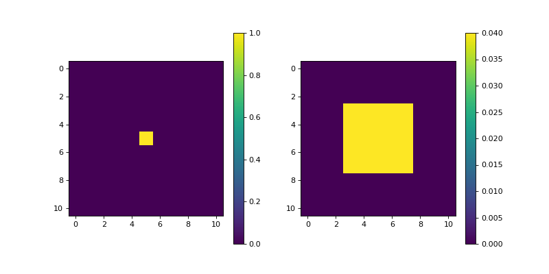
- MovingAverage(dim_shape, size, center=None, mode='constant', gpu=False, dtype=None)[source]#
Multi-dimensional moving average or uniform filter.
Notes
This operator performs a convolution between the input \(D\)-dimensional NDArray \(\mathbf{x} \in \mathbb{R}^{N_0 \times \cdots \times N_{D-1}}\) and a uniform \(D\)-dimensional filter \(\mathbf{h} \in \mathbb{R}^{\text{size} \times \cdots \times \text{size}}\) that computes the
size-point local mean values using separable kernels for improved performance.\[y_{i} = \frac{1}{|\mathcal{N}_{i}|}\sum_{j \in \mathcal{N}_{i}} x_{j}\]Where \(\mathcal{N}_{i}\) is the set of elements neighbouring the \(i\)-th element of the input array, and \(\mathcal{N}_{i}\) denotes its cardinality, i.e. the total number of neighbors.
- Parameters:
dim_shape (
NDArrayShape) – Shape of the input array.Size of the moving average kernel.
If a single integer value is provided, then the moving average filter will have as many dimensions as the input array. If a tuple is provided, it should contain as many elements as
dim_shape. For example, thesize=(1, 3)will convolve the input image with the filter[[1, 1, 1]] / 3.center (
IndexSpec) –(i_1, …, i_D) index of the kernel’s center.
centerdefines how a kernel is overlaid on inputs to produce outputs. For oddsize, it defaults to the central element (center=size//2). For evensizethe desired center indices must be provided.mode (
str,list[str]) –Boundary conditions. Multiple forms are accepted:
str: unique mode shared amongst dimensions. Must be one of:
’constant’ (default): zero-padding
’wrap’
’reflect’
’symmetric’
’edge’
tuple[str, …]: the
d-th dimension usesmode[d]as boundary condition.
(See
numpy.pad()for details.)gpu (
bool) – Input NDArray type (Truefor GPU,Falsefor CPU). Defaults toFalse.dtype (
DType) – Working precision of the linear operator.
- Returns:
op – MovingAverage
- Return type:
Example
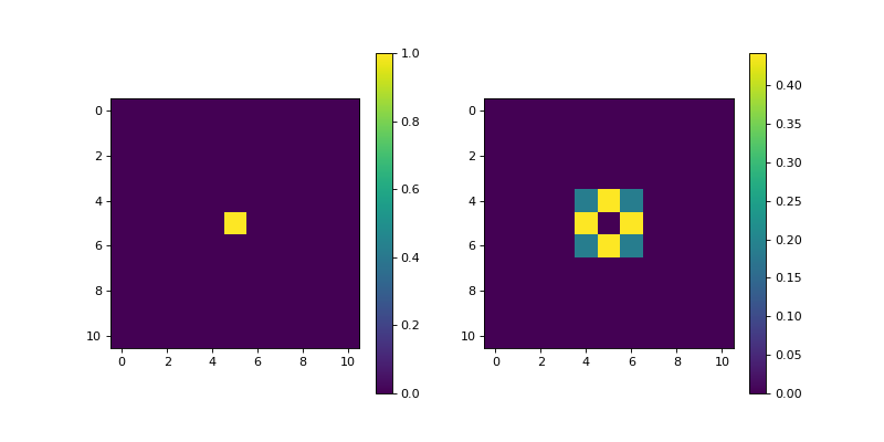
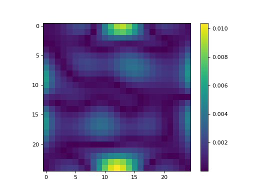
import matplotlib.pyplot as plt
import numpy as np
from pyxu.operator import MovingAverage

dim_shape = (11, 11)
image = np.zeros(dim_shape)
image[5, 5] = 1.

ma = MovingAverage(dim_shape, size=5)
out = ma(image)
plt.figure(figsize=(10, 5))
plt.subplot(121)
plt.imshow(image)
plt.colorbar()
plt.subplot(122)
plt.imshow(out)
plt.colorbar()
(
Source code,png,hires.png,pdf)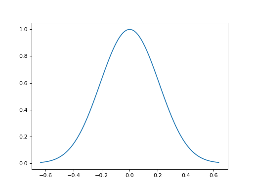
See also
GaussianFilter
- Gaussian(dim_shape)[source]#
Gaussian, element-wise.
Notes
\(f(x) = \exp(-x^{2})\)
\(f'(x) = -2 x \exp(-x^{2})\)
\(\vert f(x) - f(y) \vert \le L \vert x - y \vert\), with Lipschitz constant \(L = \sqrt{2 / e}\).
(Reason: \(\vert f'(x) \vert\) is bounded by \(L\) at \(x = \pm 1 / \sqrt{2}\).)
\(\vert f'(x) - f'(y) \vert \le \partial L \vert x - y \vert\), with diff-Lipschitz constant \(\partial L = 2\).
(Reason: \(\vert f''(x) \vert\) is bounded by \(\partial L\) at \(x = 0\).)
- DifferenceOfGaussians(
- dim_shape,
- low_sigma=1.0,
- high_sigma=None,
- low_truncate=3.0,
- high_truncate=3.0,
- mode='constant',
- sampling=1,
- gpu=False,
- dtype=None,
Multi-dimensional Difference of Gaussians filter.
Notes
This operator uses the Difference of Gaussians (DoG) method to a \(D\)-dimensional NDArray \(\mathbf{x} \in \mathbb{R}^{N_0 \times \cdots \times N_{D-1}}\) using separable kernels for improved performance. The DoG method blurs the input image with two Gaussian kernels with different sigma, and subtracts the more-blurred signal from the less-blurred image. This creates an output signal containing only the information from the original signal at the spatial scale indicated by the two sigmas.
- Parameters:
dim_shape (
NDArrayShape) – Shape of the input array.Standard deviation of the Gaussian kernel with smaller sigmas across all axes.
If a scalar value is provided, then the Gaussian filter will have as many dimensions as the input array. If a tuple is provided, it should contain as many elements as
dim_shape. Use0to prevent filtering in a given dimension. For example, thelow_sigma=(0, 3)will convolve the input image in its last dimension.high_sigma (
float,tuple,None) – Standard deviation of the Gaussian kernel with larger sigmas across all axes. IfNoneis given (default), sigmas for all axes are calculated as1.6 * low_sigma.low_truncate (
float,tuple) – Truncate the filter at this many standard deviations. Defaults to 3.0.high_truncate (
float,tuple) – Truncate the filter at this many standard deviations. Defaults to 3.0.mode (
str,list[str]) –Boundary conditions. Multiple forms are accepted:
str: unique mode shared amongst dimensions. Must be one of:
’constant’ (default): zero-padding
’wrap’
’reflect’
’symmetric’
’edge’
tuple[str, …]: the
d-th dimension usesmode[d]as boundary condition.
(See
numpy.pad()for details.)sampling (
Real,list[Real]) – Sampling step (i.e. distance between two consecutive elements of an array). Defaults to 1.gpu (
bool) – Input NDArray type (Truefor GPU,Falsefor CPU). Defaults toFalse.dtype (
DType) – Working precision of the linear operator.
- Returns:
op – DifferenceOfGaussians
- Return type:
Example
import matplotlib.pyplot as plt
import numpy as np
from pyxu.operator import DoG

dim_shape = (11, 11)
image = np.zeros(dim_shape)
image[5, 5] = 1.

dog = DoG(dim_shape, low_sigma=3)
out = dog(image)
plt.figure(figsize=(10, 5))
plt.subplot(121)
plt.imshow(image)
plt.colorbar()
plt.subplot(122)
plt.imshow(out)
plt.colorbar()
(
Source code,png,hires.png,pdf)
See also
- DoG(dim_shape, low_sigma=1.0, high_sigma=None, low_truncate=3.0, high_truncate=3.0, mode='constant', sampling=1, gpu=False, dtype=None)#
Alias of
DifferenceOfGaussians().
- Laplace(dim_shape, mode='constant', sampling=1, gpu=False, dtype=None)[source]#
Multi-dimensional Laplace filter.
The implementation is based on second derivatives approximated via finite differences.
Notes
This operator uses the applies the Laplace kernel \([1 -2 1]\) to a \(D\)-dimensional NDArray \(\mathbf{x} \in \mathbb{R}^{N_0 \times \cdots \times N_{D-1}}\) using separable kernels for improved performance. The Laplace filter is commonly used to find high-frequency components in the signal, such as for example, the edges in an image.
- Parameters:
dim_shape (
NDArrayShape) – Shape of the input array.mode (
str,list[str]) –Boundary conditions. Multiple forms are accepted:
str: unique mode shared amongst dimensions. Must be one of:
’constant’ (default): zero-padding
’wrap’
’reflect’
’symmetric’
’edge’
tuple[str, …]: the
d-th dimension usesmode[d]as boundary condition.
(See
numpy.pad()for details.)sampling (
Real,list[Real]) – Sampling step (i.e. distance between two consecutive elements of an array). Defaults to 1.gpu (
bool) – Input NDArray type (Truefor GPU,Falsefor CPU). Defaults toFalse.dtype (
DType) – Working precision of the linear operator.
- Returns:
op – DifferenceOfGaussians
- Return type:
Example
import matplotlib.pyplot as plt
import numpy as np
from pyxu.operator import Laplace

dim_shape = (11, 11)
image = np.zeros(dim_shape)
image[5, 5] = 1.

laplace = Laplace(dim_shape)
out = laplace(image)
plt.figure(figsize=(10, 5))
plt.subplot(121)
plt.imshow(image)
plt.colorbar()
plt.subplot(122)
plt.imshow(out)
plt.colorbar()
(
Source code,png,hires.png,pdf)
- Sobel(dim_shape, axis=None, mode='constant', sampling=1, gpu=False, dtype=None)[source]#
Multi-dimensional Sobel filter.
Notes
This operator uses the applies the multi-dimensional Sobel filter to a \(D\)-dimensional NDArray \(\mathbf{x} \in \mathbb{R}^{N_0 \times \cdots \times N_{D-1}}\) using separable kernels for improved performance. The Sobel filter applies the following edge filter in the dimensions of interest:
[1, 0, -1]and the smoothing filter on the rest of dimensions:[1, 2, 1] / 4. The Sobel filter is commonly used to find high-frequency components in the signal, such as for example, the edges in an image.- Parameters:
dim_shape (
NDArrayShape) – Shape of the input array.Compute the edge filter along this axis. If not provided, the edge magnitude is computed.
This is defined as:
np.sqrt(sum([sobel(array, axis=i)**2 for i in range(array.ndim)]) / array.ndim)The magnitude is also computed if axis is a sequence.mode (
str,list[str]) –Boundary conditions. Multiple forms are accepted:
str: unique mode shared amongst dimensions. Must be one of:
’constant’ (default): zero-padding
’wrap’
’reflect’
’symmetric’
’edge’
tuple[str, …]: the
d-th dimension usesmode[d]as boundary condition.
(See
numpy.pad()for details.)sampling (
Real,list[Real]) – Sampling step (i.e. distance between two consecutive elements of an array). Defaults to 1.gpu (
bool) – Input NDArray type (Truefor GPU,Falsefor CPU). Defaults toFalse.dtype (
DType) – Working precision of the linear operator.
- Returns:
op – Sobel
- Return type:
Example
import matplotlib.pyplot as plt
import numpy as np
from pyxu.operator import Sobel

dim_shape = (11, 11)
image = np.zeros(dim_shape)
image[5, 5] = 1.

sobel = Sobel(dim_shape)
out = sobel(image)
plt.figure(figsize=(10, 5))
plt.subplot(121)
plt.imshow(image)
plt.colorbar()
plt.subplot(122)
plt.imshow(out)
plt.colorbar()
(
Source code,png,hires.png,pdf)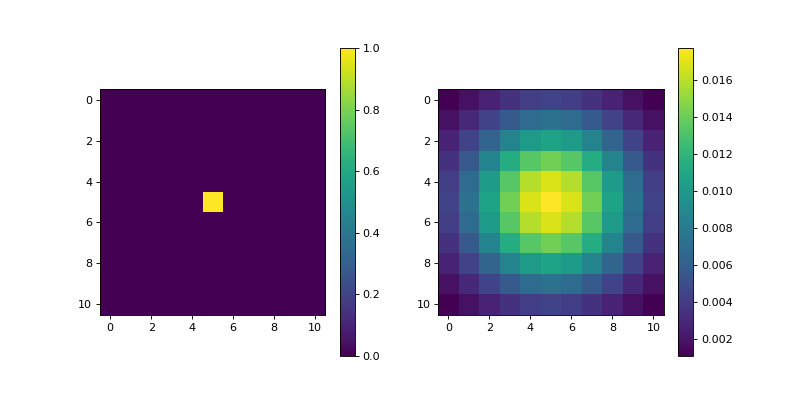
- Prewitt(dim_shape, axis=None, mode='constant', sampling=1, gpu=False, dtype=None)[source]#
Multi-dimensional Prewitt filter.
Notes
This operator uses the applies the multi-dimensional Prewitt filter to a \(D\)-dimensional NDArray \(\mathbf{x} \in \mathbb{R}^{N_0 \times \cdots \times N_{D-1}}\) using separable kernels for improved performance. The Prewitt filter applies the following edge filter in the dimensions of interest:
[1, 0, -1], and the smoothing filter on the rest of dimensions:[1, 1, 1] / 3. The Prewitt filter is commonly used to find high-frequency components in the signal, such as for example, the edges in an image.- Parameters:
dim_shape (
NDArrayShape) – Shape of the input array.Compute the edge filter along this axis. If not provided, the edge magnitude is computed. This is defined as:
np.sqrt(sum([prewitt(array, axis=i)**2 for i in range(array.ndim)]) / array.ndim)The magnitude is also computed if axis is a sequence.mode (
str,list[str]) –Boundary conditions. Multiple forms are accepted:
str: unique mode shared amongst dimensions. Must be one of:
’constant’ (default): zero-padding
’wrap’
’reflect’
’symmetric’
’edge’
tuple[str, …]: the
d-th dimension usesmode[d]as boundary condition.
(See
numpy.pad()for details.)sampling (
Real,list[Real]) – Sampling step (i.e. distance between two consecutive elements of an array). Defaults to 1.gpu (
bool) – Input NDArray type (Truefor GPU,Falsefor CPU). Defaults toFalse.dtype (
DType) – Working precision of the linear operator.
- Returns:
op – Prewitt
- Return type:
Example
import matplotlib.pyplot as plt
import numpy as np
from pyxu.operator import Prewitt

dim_shape = (11, 11)
image = np.zeros(dim_shape)
image[5, 5] = 1.

prewitt = Prewitt(dim_shape)
out = prewitt(image)
plt.figure(figsize=(10, 5))
plt.subplot(121)
plt.imshow(image)
plt.colorbar()
plt.subplot(122)
plt.imshow(out)
plt.colorbar()
(
Source code,png,hires.png,pdf)
- Scharr(dim_shape, axis=None, mode='constant', sampling=1, gpu=False, dtype=None)[source]#
Multi-dimensional Scharr filter.
Notes
This operator uses the applies the multi-dimensional Scharr filter to a \(D\)-dimensional NDArray \(\mathbf{x} \in \mathbb{R}^{N_0 \times \cdots \times N_{D-1}}\) using separable kernels for improved performance. The Scharr filter applies the following edge filter in the dimensions of interest:
[1, 0, -1], and the smoothing filter on the rest of dimensions:[3, 10, 3] / 16. The Scharr filter is commonly used to find high-frequency components in the signal, such as for example, the edges in an image.- Parameters:
dim_shape (
NDArrayShape) – Shape of the input array.Compute the edge filter along this axis. If not provided, the edge magnitude is computed. This is defined as:
np.sqrt(sum([scharr(array, axis=i)**2 for i in range(array.ndim)]) / array.ndim)The magnitude is also computed if axis is a sequence.mode (
str,list[str]) –Boundary conditions. Multiple forms are accepted:
str: unique mode shared amongst dimensions. Must be one of:
’constant’ (default): zero-padding
’wrap’
’reflect’
’symmetric’
’edge’
tuple[str, …]: the
d-th dimension usesmode[d]as boundary condition.
(See
numpy.pad()for details.)sampling (
Real,list[Real]) – Sampling step (i.e. distance between two consecutive elements of an array). Defaults to 1.gpu (
bool) – Input NDArray type (Truefor GPU,Falsefor CPU). Defaults toFalse.dtype (
DType) – Working precision of the linear operator.
- Returns:
op – Scharr
- Return type:
Example
import matplotlib.pyplot as plt
import numpy as np
from pyxu.operator import Scharr

dim_shape = (11, 11)
image = np.zeros(dim_shape)
image[5, 5] = 1.

scharr = Scharr(dim_shape)
out = scharr(image)
plt.figure(figsize=(10, 5))
plt.subplot(121)
plt.imshow(image)
plt.colorbar()
plt.subplot(122)
plt.imshow(out)
plt.colorbar()
(
Source code,png,hires.png,pdf)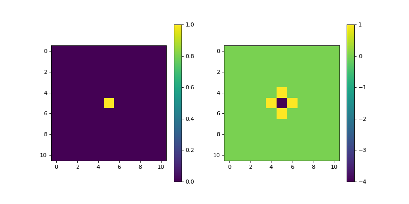
- class StructureTensor(
- dim_shape,
- diff_method='fd',
- smooth_sigma=1.0,
- smooth_truncate=3.0,
- mode='constant',
- sampling=1,
- gpu=False,
- dtype=None,
- parallel=False,
- **diff_kwargs,
Bases:
DiffMapStructure tensor operator.
Notes
The Structure Tensor, also known as the second-order moment tensor or the inertia tensor, is a matrix derived from the gradient of a function. It describes the distribution of the gradient (i.e., its prominent directions) in a specified neighbourhood around a point, and the degree to which those directions are coherent. The structure tensor of a \(D\)-dimensional signal \(\mathbf{f} \in \mathbb{R}^{N_0 \times \cdots \times N_{D-1}}\) can be written as:
\[\begin{split}\mathbf{S}_\sigma \mathbf{f} = \mathbf{g}_{\sigma} * \nabla\mathbf{f} (\nabla\mathbf{f})^{\top} = \mathbf{g}_{\sigma} * \begin{bmatrix} \left( \dfrac{ \partial\mathbf{f} }{ \partial x_{0} } \right)^2 & \dfrac{ \partial^{2}\mathbf{f} }{ \partial x_{0}\,\partial x_{1} } & \cdots & \dfrac{ \partial\mathbf{f} }{ \partial x_{0} } \dfrac{ \partial\mathbf{f} }{ \partial x_{D-1} } \\ \dfrac{ \partial\mathbf{f} }{ \partial x_{1} } \dfrac{ \partial\mathbf{f} }{ \partial x_{0} } & \left( \dfrac{ \partial\mathbf{f} }{ \partial x_{1} }\right)^2 & \cdots & \dfrac{ \partial\mathbf{f} }{ \partial x_{1} } \dfrac{ \partial\mathbf{f} }{ \partial x_{D-1} } \\ \vdots & \vdots & \ddots & \vdots \\ \dfrac{ \partial\mathbf{f} }{ \partial x_{D-1} } \dfrac{ \partial\mathbf{f} }{ \partial x_{0} } & \dfrac{ \partial\mathbf{f} }{ \partial x_{D-1} } \dfrac{ \partial\mathbf{f} }{ \partial x_{1} } & \cdots & \left( \dfrac{ \partial\mathbf{f} }{ \partial x_{D-1}} \right)^2 \end{bmatrix},\end{split}\]where \(\mathbf{g}_{\sigma} \in \mathbb{R}^{N_0 \times \cdots \times N_{D-1}}\) is a discrete Gaussian filter with standard variation \(\sigma\) with which a convolution is performed elementwise.
However, due to the symmetry of the structure tensor, only the upper triangular part is computed in practice:
\[\begin{split}\mathbf{H}_{\mathbf{v}_1, \ldots ,\mathbf{v}_m} \mathbf{f} = \mathbf{g}_{\sigma} * \begin{bmatrix} \left( \dfrac{ \partial\mathbf{f} }{ \partial x_{0} } \right)^2 \\ \dfrac{ \partial^{2}\mathbf{f} }{ \partial x_{0}\,\partial x_{1} } \\ \vdots \\ \left( \dfrac{ \partial\mathbf{f} }{ \partial x_{D-1}} \right)^2 \end{bmatrix} \mathbf{f} \in \mathbb{R}^{\frac{D (D-1)}{2} \times N_0 \times \cdots \times N_{D-1}}\end{split}\]Remark#
In case of using the finite differences (
diff_type="fd"), the finite difference scheme defaults tocentral(seePartialDerivative).Example
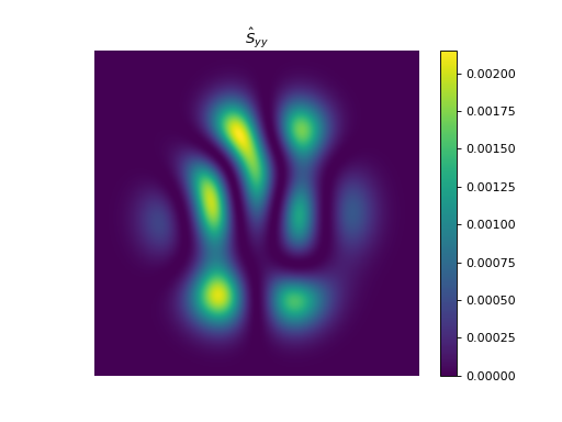
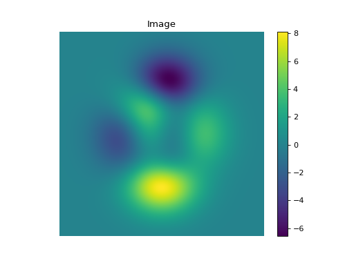
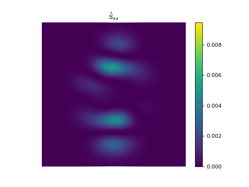
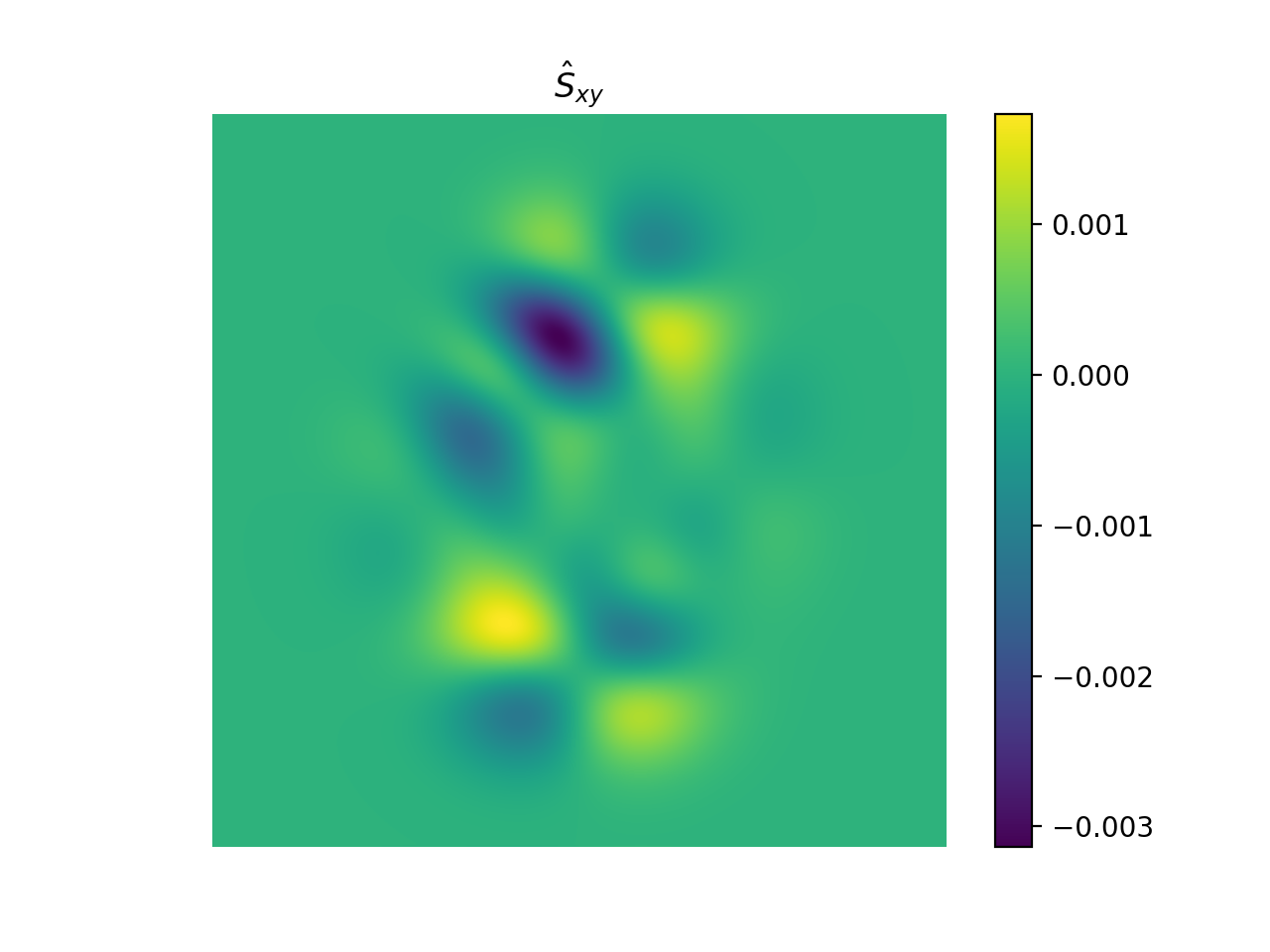
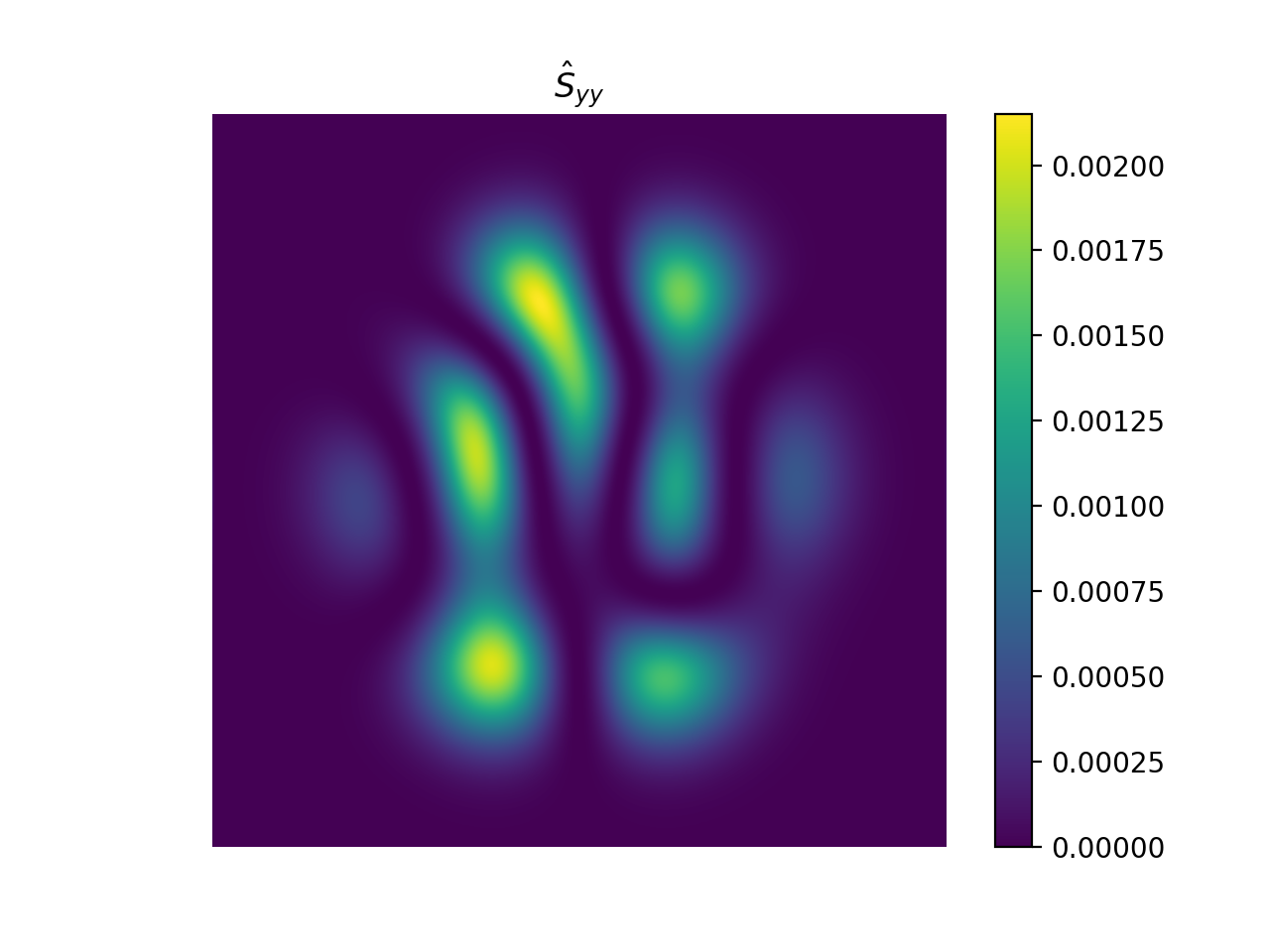
import numpy as np
import matplotlib.pyplot as plt
from pyxu.operator import StructureTensor
from pyxu.util.misc import peaks

# Define input image
n = 1000
x = np.linspace(-3, 3, n)
xx, yy = np.meshgrid(x, x)
image = peaks(xx, yy)
nsamples = 2
dim_shape = image.shape  # (1000, 1000)
images = np.tile(image, (nsamples, 1, 1))
# Instantiate structure tensor operator
structure_tensor = StructureTensor(dim_shape=dim_shape)

outputs = structure_tensor(images)
print(outputs.shape)  # (2, 3, 1000, 1000)
# Plot
plt.figure()
plt.imshow(images[0])
plt.colorbar()
plt.title("Image")
plt.axis("off")

plt.figure()
plt.imshow(outputs[0][0])
plt.colorbar()
plt.title(r"$\hat{S}_{xx}$")
plt.axis("off")

plt.figure()
plt.imshow(outputs[0][1])
plt.colorbar()
plt.title(r"$\hat{S}_{xy}$")
plt.axis("off")

plt.figure()
plt.imshow(outputs[0][2])
plt.colorbar()
plt.title(r"$\hat{S}_{yy}$")
plt.axis("off")


See also
Derivatives#
- class PartialDerivative[source]#
Bases:
objectPartial derivative operator based on Numba stencils.
Notes
This operator approximates the partial derivative of a \(D\)-dimensional signal \(\mathbf{f} \in \mathbb{R}^{N_0 \times \cdots \times N_{D-1}}\)
\[\frac{\partial^{n} \mathbf{f}}{\partial x_0^{n_0} \cdots \partial x_{D-1}^{n_{D-1}}} \in \mathbb{R}^{N_0 \times \cdots \times N_{D-1}}\]where \(\frac{\partial^{n_i}}{\partial x_i^{n_i}}\) is the \(n_i\)-th order partial derivative along dimension \(i\) and \(n = \prod_{i=0}^{D-1} n_{i}\) is the total derivative order.
Partial derivatives can be implemented with finite differences via the
finite_difference()constructor, or with the Gaussian derivative via thegaussian_derivative()constructor.When using the
finite_difference()constructor, the adjoint of the resulting linear operator will vary depending on the type of finite differences:For
forwardtype, the adjoint corresponds to:\((\frac{\partial^{\text{fwd}}}{\partial x})^{\ast} = -\frac{\partial^{\text{bwd}}}{\partial x}\)
For
backwardtype, the adjoint corresponds to:\((\frac{\partial^{\text{bwd}}}{\partial x})^{\ast} = -\frac{\partial^{\text{fwd}}}{\partial x}\)
For
centraltype, and for thegaussian_derivative()constructor, the adjoint corresponds to:\((\frac{\partial}{\partial x})^{\ast} = -\frac{\partial}{\partial x}\)
Warning
When dealing with high-order partial derivatives, the stencils required to compute them can become large, resulting in computationally expensive evaluations. In such scenarios, it can be more efficient to construct the partial derivative through a composition of lower-order partial derivatives.
- static finite_difference(dim_shape, order, scheme='forward', accuracy=1, mode='constant', gpu=False, dtype=None, sampling=1)[source]#
Compute partial derivatives for multi-dimensional signals using finite differences.
- Parameters:
dim_shape (
NDArrayShape) – (N_1,…,N_D) input dimensions.order (
list[Integer]) – Derivative order for each dimension. The total order of the partial derivative is the sum of the elements of the tuple. Use zeros to indicate dimensions in which the derivative should not be computed.scheme (
str,list[str]) – Type of finite differences: [‘forward, ‘backward, ‘central’]. Defaults to ‘forward’. If a string is provided, the sameschemeis assumed for all dimensions. If a tuple is provided, it should have as many elements asorder.accuracy (
Integer,list[Integer]) – Determines the number of points used to approximate the derivative with finite differences (seeNotes). Defaults to 1. If an int is provided, the sameaccuracyis assumed for all dimensions. If a tuple is provided, it should have as many elements asdim_shape.mode (
str,list[str]) –Boundary conditions. Multiple forms are accepted:
str: unique mode shared amongst dimensions. Must be one of:
’constant’ (default): zero-padding
’wrap’
’reflect’
’symmetric’
’edge’
tuple[str, …]: the
d-th dimension usesmode[d]as boundary condition.
(See
numpy.pad()for details.)gpu (
bool) – Input NDArray type (Truefor GPU,Falsefor CPU). Defaults toFalse.dtype (
DType) – Working precision of the linear operator.sampling (
Real,list[Real]) – Sampling step (i.e. distance between two consecutive elements of an array). Defaults to 1.
- Returns:
op – Partial derivative
- Return type:
Notes
We explain here finite differences for one-dimensional signals; this operator performs finite differences for multi-dimensional signals along dimensions specified by
order.This operator approximates derivatives with finite differences. It is inspired by the Finite Difference Coefficients Calculator to construct finite-difference approximations for the desired (i) derivative order, (ii) approximation accuracy, and (iii) finite difference type. Three basic types of finite differences are supported, which lead to the following first-order (
order = 1) operators withaccuracy = 1and sampling stepsampling = hfor one-dimensional signals:Forward difference: Approximates the continuous operator \(D_{F}f(x) = \frac{f(x+h) - f(x)}{h}\) with the discrete operator
\[\mathbf{D}_{F} f [n] = \frac{f[n+1] - f[n]}{h},\]whose kernel is \(d = \frac{1}{h}[-1, 1]\) and center is (0, ).
Backward difference: Approximates the continuous operator \(D_{B}f(x) = \frac{f(x) - f(x-h)}{h}\) with the discrete operator
\[\mathbf{D}_{B} f [n] = \frac{f[n] - f[n-1]}{h},\]whose kernel is \(d = \frac{1}{h}[-1, 1]\) and center is (1, ).
Central difference: Approximates the continuous operator \(D_{C}f(x) = \frac{f(x+h) - f(x-h)}{2h}\) with the discrete operator
\[\mathbf{D}_{C} f [n] = \frac{f[n+1] - f[n-1]}{2h},\]whose kernel is \(d = \frac{1}{h}[-\frac12, 0, \frac12]\) and center is (1, ).
Warning
For forward and backward differences, higher-order operators correspond to the composition of first-order operators. This is not the case for central differences: the second-order continuous operator is given by \(D^2_{C}f(x) = \frac{f(x+h) - 2 f(x) + f(x-h)}{h}\), hence \(D^2_{C} \neq D_{C} \circ D_{C}\). The corresponding discrete operator is given by \(\mathbf{D}^2_{C} f [n] = \frac{f[n+1] - 2 f[n] + f[n-1]}{h}\), whose kernel is \(d = \frac{1}{h}[1, -2, 1]\) and center is (1, ). We refer to this paper for more details.
For a given derivative order \(N\in\mathbb{Z}^{+}\) and accuracy \(a\in\mathbb{Z}^{+}\), the size \(N_s\) of the stencil kernel \(d\) used for finite differences is given by:
For central differences: \(N_s = 2 \lfloor\frac{N + 1}{2}\rfloor - 1 + a\)
For forward and backward differences: \(N_s = N + a\)
For \(N_s\) given support indices \(\{s_1, \ldots , s_{N_s} \} \subset \mathbb{Z}\) and a derivative order \(N<N_s\), the stencil kernel \(d = [d_1, \ldots, d_{N_s}]\) of the finite-difference approximation of the derivative is obtained by solving the following system of linear equations (see the Finite Difference Coefficients Calculator documentation):
Remark
The number of coefficients of the finite-difference kernel is chosen to guarantee the requested accuracy, but might be larger than requested accuracy. For example, if choosing
scheme='central'withaccuracy=1, it will create a kernel corresponding toaccuracy=2, as it is the minimum accuracy possible for such scheme (see the finite difference coefficient table).\[\begin{split}\left(\begin{array}{ccc} s_{1}^{0} & \cdots & s_{N_s}^{0} \\ \vdots & \ddots & \vdots \\ s_{1}^{N_s-1} & \cdots & s_{N_s}^{N_s-1} \end{array}\right)\left(\begin{array}{c} d_{1} \\ \vdots \\ d_{N_s} \end{array}\right)= \frac{1}{h^{N}}\left(\begin{array}{c} \delta_{0, N} \\ \vdots \\ \delta_{i, N} \\ \vdots \\ \delta_{N_s-1, N} \end{array}\right),\end{split}\]where \(\delta_{i, j}\) is the Kronecker delta.
This class inherits its methods from
Stencil.Example
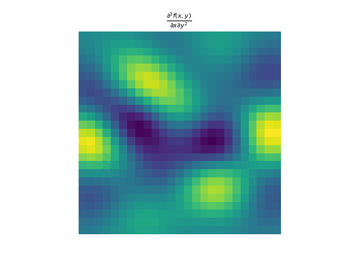
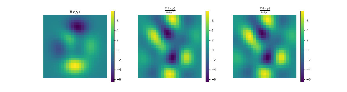
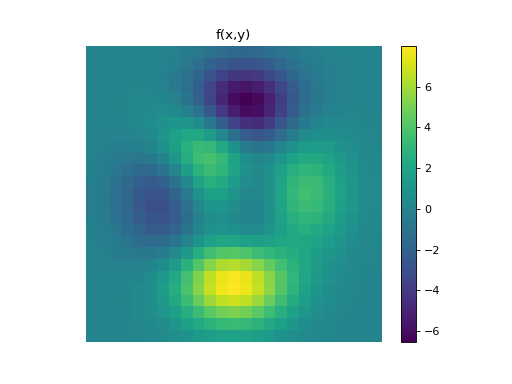
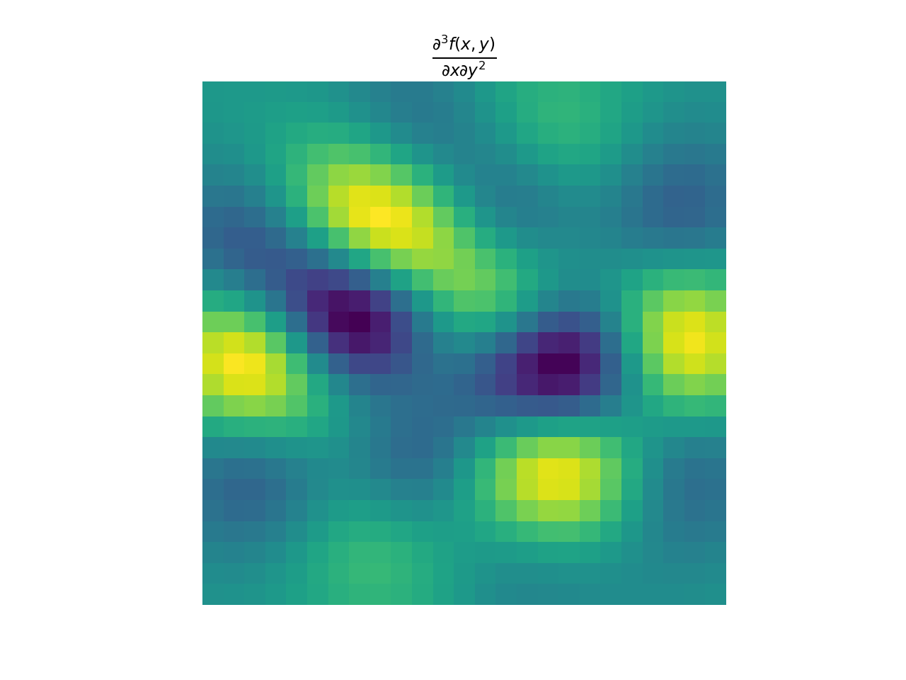
import numpy as np
import matplotlib.pyplot as plt
from pyxu.operator import PartialDerivative
from pyxu.util.misc import peaks

x = np.linspace(-2.5, 2.5, 25)
xx, yy = np.meshgrid(x, x)
image = peaks(xx, yy)
dim_shape = image.shape  # Shape of our image
# Specify derivative order at each direction
df_dx = (1, 0)  # Compute derivative of order 1 in first dimension
d2f_dy2 = (0, 2)  # Compute derivative of order 2 in second dimension
d3f_dxdy2 = (1, 2)  # Compute derivative of order 1 in first dimension and der. of order 2 in second dimension
# Instantiate derivative operators
sigma = 2.0
diff1 = PartialDerivative.gaussian_derivative(order=df_dx, dim_shape=dim_shape, sigma=sigma / np.sqrt(2))
diff2 = PartialDerivative.gaussian_derivative(order=d2f_dy2, dim_shape=dim_shape, sigma=sigma / np.sqrt(2))
diff = PartialDerivative.gaussian_derivative(order=d3f_dxdy2, dim_shape=dim_shape, sigma=sigma)
# Compute derivatives
out1 = (diff1 * diff2)(image)
out2 = diff(image)
# Plot derivatives
fig, axs = plt.subplots(1, 3, figsize=(15, 4))
im = axs[0].imshow(image)
axs[0].axis("off")
axs[0].set_title("f(x,y)")
plt.colorbar(im, ax=axs[0])
axs[1].imshow(out1)
axs[1].axis("off")
axs[1].set_title(r"$\frac{\partial^{3} f(x,y)}{\partial x\partial y^{2}}$")
plt.colorbar(im, ax=axs[1])

axs[2].imshow(out2)
axs[2].axis("off")
axs[2].set_title(r"$\frac{\partial^{3} f(x,y)}{\partial x\partial y^{2}}$")
plt.colorbar(im, ax=axs[2])

# Check approximation error
plt.figure()
plt.imshow(abs(out1 - out2)), plt.colorbar()

- static gaussian_derivative(dim_shape, order, sigma=1.0, truncate=3.0, mode='constant', gpu=False, dtype=None, sampling=1)[source]#
Compute partial derivatives for multi-dimensional signals using gaussian derivatives.
- Parameters:
dim_shape (
NDArrayShape) – (N_1,…,N_D) input dimensions.order (
list[Integer]) – Derivative order for each dimension. The total order of the partial derivative is the sum of the elements of the tuple. Use zeros to indicate dimensions in which the derivative should not be computed.sigma (
Real,list[Real]) – Standard deviation for the Gaussian kernel. Defaults to 1.0. If a float is provided, the samesigmais assumed for all dimensions. If a tuple is provided, it should have as many elements asorder.truncate (
Real,list[Real]) – Truncate the filter at this many standard deviations (at each side from the origin). Defaults to 3.0. If a float is provided, the sametruncateis assumed for all dimensions. If a tuple is provided, it should have as many elements asorder.mode (
str,list[str]) –Boundary conditions. Multiple forms are accepted:
str: unique mode shared amongst dimensions. Must be one of:
’constant’ (default): zero-padding
’wrap’
’reflect’
’symmetric’
’edge’
tuple[str, …]: the
d-th dimension usesmode[d]as boundary condition.
(See
numpy.pad()for details.)gpu (
bool) – Input NDArray type (Truefor GPU,Falsefor CPU). Defaults toFalse.dtype (
DType) – Working precision of the linear operator.sampling (
Real,list[Real]) – Sampling step (i.e., the distance between two consecutive elements of an array). Defaults to 1.
- Returns:
op – Partial derivative.
- Return type:
Notes
We explain here Gaussian derivatives for one-dimensional signals; this operator performs partial Gaussian derivatives for multi-dimensional signals along dimensions specified by
order.A Gaussian derivative is an approximation of a derivative that consists in convolving the input function with a Gaussian function \(g\) before applying a derivative. In the continuous domain, the \(N\)-th order Gaussian derivative \(D^N_G\) amounts to a convolution with the \(N\)-th order derivative of \(g\):
\[D^N_G f (x) = \frac{\mathrm{d}^N (f * g) }{\mathrm{d} x^N} (x) = f(x) * \frac{\mathrm{d}^N g}{\mathrm{d} x^N} (x).\]For discrete signals \(f[n]\), this operator is approximated by
\[\mathbf{D}^N_G f [n] = f[n] *\frac{\mathrm{d}^N g}{\mathrm{d} x^N} \left(\frac{n}{h}\right),\]where \(h\) is the spacing between samples and the operator \(*\) is now a discrete convolution.
Warning
The operator \(\mathbf{D}_{G} \circ \mathbf{D}_{G}\) is not directly related to \(\mathbf{D}_{G}^{2}\): Gaussian smoothing is performed twice in the case of the former, whereas it is performed only once in the case of the latter.
Note that in contrast with finite differences (see
finite_difference()), Gaussian derivatives compute exact derivatives in the continuous domain, since Gaussians can be differentiated analytically. This derivative is then sampled in order to perform a discrete convolution.This class inherits its methods from
Stencil.Example
import numpy as np
import matplotlib.pyplot as plt
from pyxu.operator import PartialDerivative
from pyxu.util.misc import peaks

x = np.linspace(-2.5, 2.5, 25)
xx, yy = np.meshgrid(x, x)
image = peaks(xx, yy)
dim_shape = image.shape  # Shape of our image
# Specify derivative order at each direction
df_dx = (1, 0) # Compute derivative of order 1 in first dimension
d2f_dy2 = (0, 2) # Compute derivative of order 2 in second dimension
d3f_dxdy2 = (1, 2) # Compute derivative of order 1 in first dimension and der. of order 2 in second dimension
# Instantiate derivative operators
diff1 = PartialDerivative.gaussian_derivative(order=df_dx, dim_shape=dim_shape, sigma=2.0)
diff2 = PartialDerivative.gaussian_derivative(order=d2f_dy2, dim_shape=dim_shape, sigma=2.0)
diff = PartialDerivative.gaussian_derivative(order=d3f_dxdy2, dim_shape=dim_shape, sigma=2.0)
# Compute derivatives
out1 = (diff1 * diff2)(image)
out2 = diff(image)
plt.figure()
plt.imshow(image),
plt.axis('off')
plt.colorbar()
plt.title('f(x,y)')
plt.figure()
plt.imshow(out1.T)
plt.axis('off')
plt.title(r'$\frac{\partial^{3} f(x,y)}{\partial x\partial y^{2}}$')
plt.figure()
plt.imshow(out2.T)
plt.axis('off')
plt.title(r'$\frac{\partial^{3} f(x,y)}{\partial x\partial y^{2}}$')


- Gradient(dim_shape, directions=None, diff_method='fd', mode='constant', gpu=False, dtype=None, **diff_kwargs)[source]#
Gradient operator.
Notes
This operator stacks the first-order partial derivatives of a \(D\)-dimensional signal \(\mathbf{f} \in \mathbb{R}^{N_{0} \times \cdots \times N_{D-1}}\) along each dimension:
\[\begin{split}\boldsymbol{\nabla} \mathbf{f} = \begin{bmatrix} \frac{\partial \mathbf{f}}{\partial x_0} \\ \vdots \\ \frac{\partial \mathbf{f}}{\partial x_{D-1}} \end{bmatrix} \in \mathbb{R}^{D \times N_{0} \times \cdots \times N_{D-1}}\end{split}\]The partial derivatives can be approximated by finite differences via the
finite_difference()constructor or by the Gaussian derivative viagaussian_derivative()constructor. The parametrization of the partial derivatives can be done via the keyword arguments**diff_kwargs, which will default to the same values as thePartialDerivativeconstructor.- Parameters:
dim_shape (
NDArrayShape) – (N_1,…,N_D) input dimensions.directions (
Integer,list[Integer],None) – Gradient directions. Defaults toNone, which computes the gradient for all directions.diff_method (
'gd','fd') –Method used to approximate the derivative. Must be one of:
’fd’ (default): finite differences
’gd’: Gaussian derivative
mode (
str,list[str]) –Boundary conditions. Multiple forms are accepted:
str: unique mode shared amongst dimensions. Must be one of:
’constant’ (default): zero-padding
’wrap’
’reflect’
’symmetric’
’edge’
tuple[str, …]: the
d-th dimension usesmode[d]as boundary condition.
(See
numpy.pad()for details.)gpu (
bool) – Input NDArray type (Truefor GPU,Falsefor CPU). Defaults toFalse.dtype (
DType) – Working precision of the linear operator.diff_kwargs (
dict) – Keyword arguments to parametrize partial derivatives (seefinite_difference()andgaussian_derivative())
- Returns:
op – Gradient
- Return type:
Example
import numpy as np
import matplotlib.pyplot as plt
from pyxu.operator import Gradient
from pyxu.util.misc import peaks

# Define input image
n = 100
x = np.linspace(-3, 3, n)
xx, yy = np.meshgrid(x, x)
image = peaks(xx, yy)
dim_shape = image.shape  # (1000, 1000)
# Instantiate gradient operator
grad = Gradient(dim_shape=dim_shape)

# Compute gradients
df_dx, df_dy = grad(image) # shape = (2, 1000, 1000)

# Plot image
fig, axs = plt.subplots(1, 3, figsize=(15, 4))
im = axs[0].imshow(image)
axs[0].set_title("Image")
axs[0].axis("off")
plt.colorbar(im, ax=axs[0])

# Plot gradient
im = axs[1].imshow(df_dx)
axs[1].set_title(r"$\partial f/ \partial x$")
axs[1].axis("off")
plt.colorbar(im, ax=axs[1])
im = axs[2].imshow(df_dy)
axs[2].set_title(r"$\partial f/ \partial y$")
axs[2].axis("off")
plt.colorbar(im, ax=axs[2])
(
Source code,png,hires.png,pdf)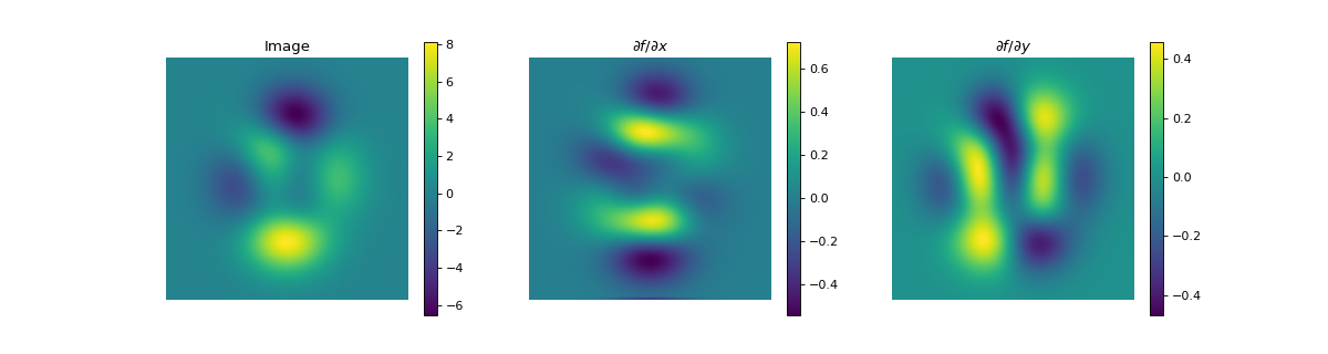
See also
- Jacobian(dim_shape, directions=None, diff_method='fd', mode='constant', gpu=False, dtype=None, **diff_kwargs)[source]#
Jacobian operator.
Notes
This operator computes the first-order partial derivatives of a \(D\)-dimensional vector-valued signal of \(C\) variables or channels \(\mathbf{f} = [\mathbf{f}_{0}, \ldots, \mathbf{f}_{C-1}]\) with \(\mathbf{f}_{c} \in \mathbb{R}^{N_{0} \times \cdots \times N_{D-1}}\).
The Jacobian of \(\mathbf{f}\) is computed via the gradient as follows:
\[\begin{split}\mathbf{J} \mathbf{f} = \begin{bmatrix} (\boldsymbol{\nabla} \mathbf{f}_{0})^{\top} \\ \vdots \\ (\boldsymbol{\nabla} \mathbf{f}_{C-1})^{\top} \\ \end{bmatrix} \in \mathbb{R}^{C \times D \times N_0 \times \cdots \times N_{D-1}}\end{split}\]The partial derivatives can be approximated by finite differences via the
finite_difference()constructor or by the Gaussian derivative viagaussian_derivative()constructor. The parametrization of the partial derivatives can be done via the keyword arguments**diff_kwargs, which will default to the same values as thePartialDerivativeconstructor.Remark
Pyxu’s convention when it comes to field-vectors, is to work with vectorized arrays. However, the memory order of these arrays should be
[S_0, ..., S_B, C, N_1, ..., N_D]shape, withS_0, ..., S_Bbeing stacking or batching dimensions,Cbeing the number of variables or channels, andN_ibeing the size of thei-th axis of the domain.- Parameters:
dim_shape (
NDArrayShape) – (C, N_1,…,N_D) input dimensions.directions (
Integer,list[Integer],None) – Gradient directions. Defaults toNone, which computes the gradient for all directions.diff_method (
"gd","fd") –Method used to approximate the derivative. Must be one of:
’fd’ (default): finite differences
’gd’: Gaussian derivative
mode (
str,list[str]) –Boundary conditions. Multiple forms are accepted:
str: unique mode shared amongst dimensions. Must be one of:
’constant’ (default): zero-padding
’wrap’
’reflect’
’symmetric’
’edge’
tuple[str, …]: the
d-th dimension usesmode[d]as boundary condition.
(See
numpy.pad()for details.)gpu (
bool) – Input NDArray type (Truefor GPU,Falsefor CPU). Defaults toFalse.dtype (
DType) – Working precision of the linear operator.diff_kwargs (
dict) – Keyword arguments to parametrize partial derivatives (seefinite_difference()andgaussian_derivative())
- Returns:
op – Jacobian
- Return type:
Example
import numpy as np
import matplotlib.pyplot as plt
from pyxu.operator import Jacobian
from pyxu.util.misc import peaks

x = np.linspace(-2.5, 2.5, 25)
xx, yy = np.meshgrid(x, x)
image = np.tile(peaks(xx, yy), (3, 1, 1))
jac = Jacobian(dim_shape=image.shape)
out = jac(image)
fig, axes = plt.subplots(3, 2, figsize=(10, 15))
for i in range(3):
   for j in range(2):
       axes[i, j].imshow(out[i, j].T, cmap=["Reds", "Greens", "Blues"][i])
       axes[i, j].set_title(f"$\partial I_{{{['R', 'G', 'B'][j]}}}/\partial{{{['x', 'y'][j]}}}$")
plt.suptitle("Jacobian")
(
Source code,png,hires.png,pdf)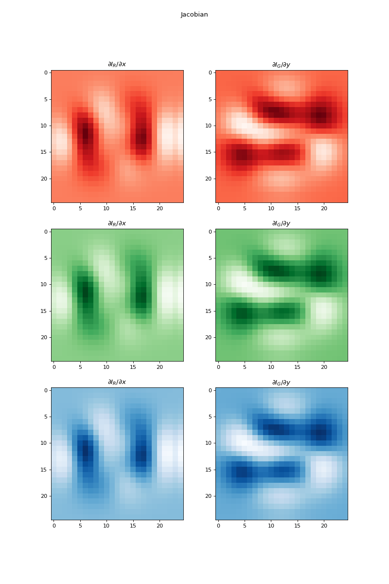
See also
- Divergence(dim_shape, directions=None, diff_method='fd', mode='constant', gpu=False, dtype=None, **diff_kwargs)[source]#
Divergence operator.
Notes
This operator computes the expansion or outgoingness of a \(D\)-dimensional vector-valued signal of \(C\) variables \(\mathbf{f} = [\mathbf{f}_{0}, \ldots, \mathbf{f}_{C-1}]\) with \(\mathbf{f}_{c} \in \mathbb{R}^{N_{0} \times \cdots \times N_{D-1}}\).
The Divergence of \(\mathbf{f}\) is computed via the adjoint of the gradient as follows:
\[\operatorname{Div} \mathbf{f} = \boldsymbol{\nabla}^{\ast} \mathbf{f} = \begin{bmatrix} \frac{\partial \mathbf{f}}{\partial x_0} + \cdots + \frac{\partial \mathbf{f}}{\partial x_{D-1}} \end{bmatrix} \in \mathbb{R}^{N_{0} \times \cdots \times N_{D-1}}\]The partial derivatives can be approximated by finite differences via the
finite_difference()constructor or by the Gaussian derivative viagaussian_derivative()constructor. The parametrization of the partial derivatives can be done via the keyword arguments**diff_kwargs, which will default to the same values as thePartialDerivativeconstructor.When using finite differences to compute the Divergence (i.e.,
diff_method = "fd"), the divergence returns the adjoint of the gradient in reversed order:For
forwardtype divergence, the adjoint of the gradient of “backward” type is used.For
backwardtype divergence, the adjoint of the gradient of “forward” type is used.
For
centraltype divergence, and for the Gaussian derivative method (i.e.,diff_method = "gd"), the adjoint of the gradient of “central” type is used (no reversed order).- Parameters:
dim_shape (
NDArrayShape) – (C, N_1,…,N_D) input dimensions.directions (
Integer,list[Integer],None) – Divergence directions. Defaults toNone, which computes the divergence for all directions.diff_method (
"gd","fd") –Method used to approximate the derivative. Must be one of:
’fd’ (default): finite differences
’gd’: Gaussian derivative
mode (
str,list[str]) –Boundary conditions. Multiple forms are accepted:
str: unique mode shared amongst dimensions. Must be one of:
’constant’ (default): zero-padding
’wrap’
’reflect’
’symmetric’
’edge’
tuple[str, …]: the
d-th dimension usesmode[d]as boundary condition.
(See
numpy.pad()for details.)gpu (
bool) – Input NDArray type (Truefor GPU,Falsefor CPU). Defaults toFalse.dtype (
DType) – Working precision of the linear operator.diff_kwargs (
dict) – Keyword arguments to parametrize partial derivatives (seefinite_difference()andgaussian_derivative())
- Returns:
op – Divergence
- Return type:
Example
import numpy as np
import matplotlib.pyplot as plt
from pyxu.operator import Gradient, Divergence, Laplacian
from pyxu.util.misc import peaks

n = 100
x = np.linspace(-3, 3, n)
xx, yy = np.meshgrid(x, x)
image = peaks(xx, yy)
dim_shape = image.shape  # (1000, 1000)
grad = Gradient(dim_shape=dim_shape)
div = Divergence(dim_shape=dim_shape)
# Construct Laplacian via composition
laplacian1 = div * grad
# Compare to default Laplacian
laplacian2 = Laplacian(dim_shape=dim_shape)
output1 = laplacian1(image)
output2 = laplacian2(image)
fig, axes = plt.subplots(1, 2, figsize=(10, 5))
im = axes[0].imshow(np.log(abs(output1)).reshape(*dim_shape))
axes[0].set_title("Laplacian via composition")
plt.colorbar(im, ax=axes[0])
im = axes[1].imshow(np.log(abs(output1)).reshape(*dim_shape))
axes[1].set_title("Default Laplacian")
plt.colorbar(im, ax=axes[1])
See also
- Hessian(dim_shape, directions='all', diff_method='fd', mode='constant', gpu=False, dtype=None, **diff_kwargs)[source]#
Hessian operator.
Notes
The Hessian matrix or Hessian of a \(D\)-dimensional signal \(\mathbf{f} \in \mathbb{R}^{N_0 \times \cdots \times N_{D-1}}\) is the square matrix of second-order partial derivatives:
\[\begin{split}\mathbf{H} \mathbf{f} = \begin{bmatrix} \dfrac{ \partial^{2}\mathbf{f} }{ \partial x_{0}^{2} } & \dfrac{ \partial^{2}\mathbf{f} }{ \partial x_{0}\,\partial x_{1} } & \cdots & \dfrac{ \partial^{2}\mathbf{f} }{ \partial x_{0} \, \partial x_{D-1} } \\ \dfrac{ \partial^{2}\mathbf{f} }{ \partial x_{1} \, \partial x_{0} } & \dfrac{ \partial^{2}\mathbf{f} }{ \partial x_{1}^{2} } & \cdots & \dfrac{ \partial^{2}\mathbf{f} }{\partial x_{1} \,\partial x_{D-1}} \\ \vdots & \vdots & \ddots & \vdots \\ \dfrac{ \partial^{2}\mathbf{f} }{ \partial x_{D-1} \, \partial x_{0} } & \dfrac{ \partial^{2}\mathbf{f} }{ \partial x_{D-1} \, \partial x_{1} } & \cdots & \dfrac{ \partial^{2}\mathbf{f} }{ \partial x_{D-1}^{2}} \end{bmatrix}\end{split}\]The partial derivatives can be approximated by finite differences via the
finite_difference()constructor or by the Gaussian derivative viagaussian_derivative()constructor. The parametrization of the partial derivatives can be done via the keyword arguments**diff_kwargs, which will default to the same values as thePartialDerivativeconstructor.The Hessian being symmetric, only the upper triangular part at most needs to be computed. Due to the (possibly) large size of the full Hessian, 4 different options are handled:
[mode 0]
directionsis an integer, e.g.:directions=0\[\partial^{2}\mathbf{f}/\partial x_{0}^{2}.\][mode 1]
directionsis a tuple of length 2, e.g.:directions=(0,1)\[\partial^{2}\mathbf{f}/\partial x_{0}\partial x_{1}.\][mode 2]
directionsis a tuple of tuples, e.g.:directions=((0,0), (0,1))\[\left(\frac{ \partial^{2}\mathbf{f} }{ \partial x_{0}^{2} }, \frac{ \partial^{2}\mathbf{f} }{ \partial x_{0}\partial x_{1} }\right).\][mode 3]
directions = 'all'(default), computes the Hessian for all directions (only the upper triangular part of the Hessian matrix), in row order, i.e.:\[\left(\frac{ \partial^{2}\mathbf{f} }{ \partial x_{0}^{2} }, \frac{ \partial^{2}\mathbf{f} } { \partial x_{0}\partial x_{1} }, \, \ldots , \, \frac{ \partial^{2}\mathbf{f} }{ \partial x_{D-1}^{2} }\right).\]
The shape of the output
LinOpdepends on the number of computed directions; by default (all directions), we have \(\mathbf{H} \mathbf{f} \in \mathbb{R}^{\frac{D(D-1)}{2} \times N_0 \times \cdots \times N_{D-1}}\).- Parameters:
dim_shape (
NDArrayShape) – (N_1,…,N_D) input dimensions.directions (
Integer,(Integer,Integer),((Integer,Integer),...,(Integer,Integer)),'all') – Hessian directions. Defaults toall, which computes the Hessian for all directions. (SeeNotes.)diff_method (
"gd","fd") –Method used to approximate the derivative. Must be one of:
’fd’ (default): finite differences
’gd’: Gaussian derivative
mode (
str,list[str]) –Boundary conditions. Multiple forms are accepted:
str: unique mode shared amongst dimensions. Must be one of:
’constant’ (default): zero-padding
’wrap’
’reflect’
’symmetric’
’edge’
tuple[str, …]: the
d-th dimension usesmode[d]as boundary condition.
(See
numpy.pad()for details.)gpu (
bool) – Input NDArray type (Truefor GPU,Falsefor CPU). Defaults toFalse.dtype (
DType) – Working precision of the linear operator.diff_kwargs (
dict) – Keyword arguments to parametrize partial derivatives (seefinite_difference()andgaussian_derivative())
- Returns:
op – Hessian
- Return type:
Example
import numpy as np
import matplotlib.pyplot as plt
from pyxu.operator import Hessian, PartialDerivative
from pyxu.util.misc import peaks

n = 100
x = np.linspace(-3, 3, n)
xx, yy = np.meshgrid(x, x)
image = peaks(xx, yy)
dim_shape = image.shape  # (1000, 1000)

# Instantiate Hessian operator
hessian = Hessian(dim_shape=dim_shape, directions="all")
# Compute Hessian
d2f_dx2, d2f_dxdy, d2f_dy2 = hessian(image)

# Plot
fig, axs = plt.subplots(1, 4, figsize=(20, 4))
im = axs[0].imshow(image)
plt.colorbar(im, ax=axs[0])
axs[0].set_title("Image")
axs[0].axis("off")

im = axs[1].imshow(d2f_dx2)
plt.colorbar(im, ax=axs[1])
axs[1].set_title(r"$\partial^{2} f/ \partial x^{2}$")
axs[1].axis("off")

im = axs[2].imshow(d2f_dxdy)
plt.colorbar(im, ax=axs[2])
axs[2].set_title(r"$\partial^{2} f/ \partial x\partial y$")
axs[2].axis("off")

im = axs[3].imshow(d2f_dy2)
plt.colorbar(im, ax=axs[3])
axs[3].set_title(r"$\partial^{2} f/ \partial y^{2}$")
axs[3].axis("off")
(
Source code,png,hires.png,pdf)
See also
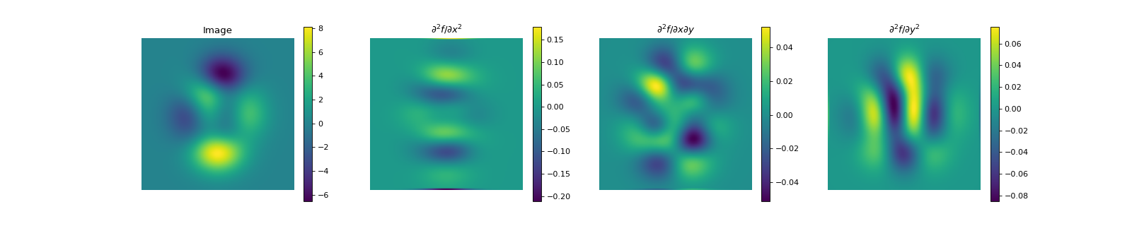
- Laplacian(dim_shape, directions=None, diff_method='fd', mode='constant', gpu=False, dtype=None, **diff_kwargs)[source]#
Laplacian operator.
Notes
The Laplacian of a \(D\)-dimensional signal \(\mathbf{f} \in \mathbb{R}^{N_0 \times \cdots \times N_{D-1}}\) is the sum of second-order partial derivatives across all input directions:
\[\sum_{d = 0}^{D-1} \dfrac{ \partial^{2}\mathbf{f} }{ \partial x_{d}^{2} }\]The partial derivatives can be approximated by finite differences via the
finite_difference()constructor or by the Gaussian derivative viagaussian_derivative()constructor. The parametrization of the partial derivatives can be done via the keyword arguments**diff_kwargs, which will default toscheme='central'andaccuracy=2fordiff_method='fd'(finite difference), and the same values as thePartialDerivativeconstructor fordiff_method='gd'(gaussian derivative).- Parameters:
dim_shape (
NDArrayShape) – (N_1,…,N_D) input dimensions.directions (
Integer,list[Integer],None) – Laplacian directions. Defaults toNone, which computes the Laplacian with all directions.diff_method (
"gd","fd") –Method used to approximate the derivative. Must be one of:
’fd’ (default): finite differences
’gd’: Gaussian derivative
mode (
str,list[str]) –Boundary conditions. Multiple forms are accepted:
str: unique mode shared amongst dimensions. Must be one of:
’constant’ (default): zero-padding
’wrap’
’reflect’
’symmetric’
’edge’
tuple[str, …]: the
d-th dimension usesmode[d]as boundary condition.
(See
numpy.pad()for details.)gpu (
bool) – Input NDArray type (Truefor GPU,Falsefor CPU). Defaults toFalse.dtype (
DType) – Working precision of the linear operator.diff_kwargs (
dict) – Keyword arguments to parametrize partial derivatives (seefinite_difference()andgaussian_derivative())
- Returns:
op – Laplacian
- Return type:
Example
import numpy as np
import matplotlib.pyplot as plt
from pyxu.operator import Laplacian
from pyxu.util.misc import peaks

# Define input image
n = 100
x = np.linspace(-3, 3, n)
xx, yy = np.meshgrid(x, x)
image = peaks(xx, yy)

dim_shape = image.shape  # (1000, 1000)
# Compute Laplacian
laplacian = Laplacian(dim_shape=dim_shape)
output = laplacian(image) # shape = (1, 1000, 1000)

# Plot
fig, axs = plt.subplots(1, 2, figsize=(10, 4))
im = axs[0].imshow(image)
plt.colorbar(im, ax=axs[0])
axs[0].set_title("Image")
axs[0].axis("off")

im = axs[1].imshow(output.squeeze())
plt.colorbar(im, ax=axs[1])
axs[1].set_title(r"$\partial^{2} f/ \partial x^{2}+\partial^{2} f/ \partial y^{2}$")
axs[1].axis("off")

fig.show()
(
Source code,png,hires.png,pdf)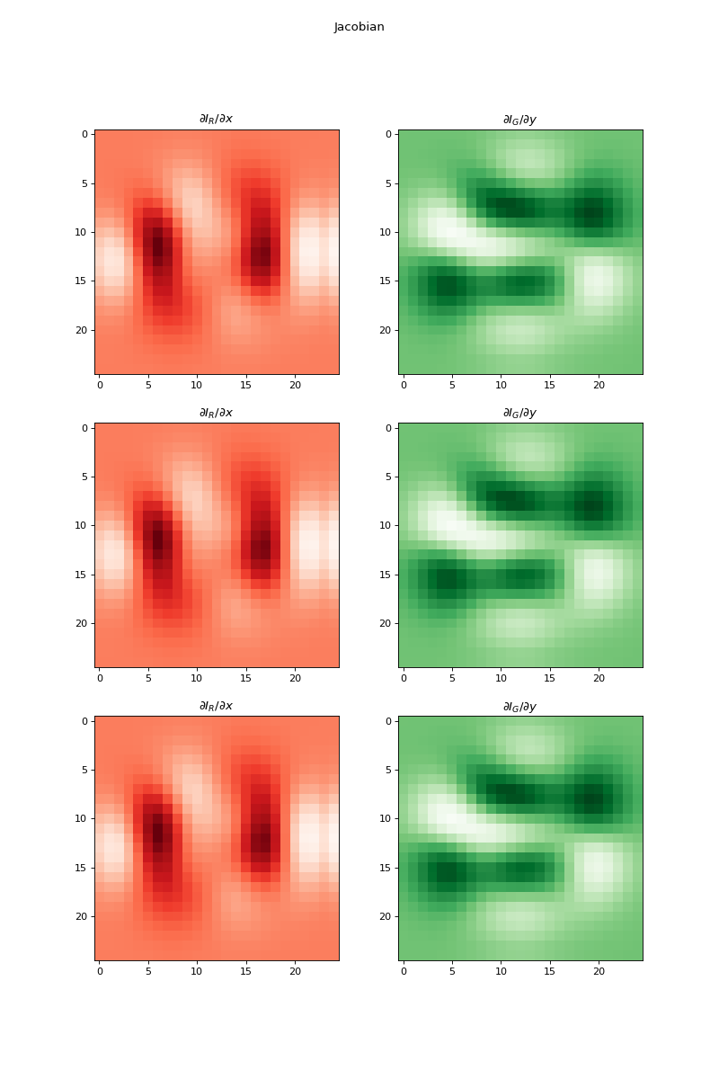
See also
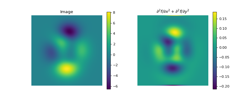
- DirectionalDerivative(dim_shape, order, directions, diff_method='fd', mode='constant', **diff_kwargs)[source]#
Directional derivative operator.
Notes
The first-order
DirectionalDerivativeof a \(D\)-dimensional signal \(\mathbf{f} \in \mathbb{R}^{N_0 \times \cdots \times N_{D-1}}\) applies a derivative along the direction specified by a constant unitary vector \(\mathbf{v} \in \mathbb{R}^D\):\[\boldsymbol{\nabla}_\mathbf{v} \mathbf{f} = \sum_{i=0}^{D-1} v_i \frac{\partial \mathbf{f}}{\partial x_i} \in \mathbb{R}^{N_0 \times \cdots \times N_{D-1}}\]or along spatially-varying directions \(\mathbf{v} = [\mathbf{v}_0, \ldots , \mathbf{v}_{D-1}]^\top \in \mathbb{R}^{D \times N_0 \times \cdots \times N_{D-1} }\) where each direction \(\mathbf{v}_{\cdot, i_0, \ldots , i_{D-1}} \in \mathbb{R}^D\) for any \(0 \leq i_d \leq N_d-1\) with \(0 \leq d \leq D-1\) is a unitary vector:
\[\boldsymbol{\nabla}_\mathbf{v} \mathbf{f} = \sum_{i=0}^{D-1} \mathbf{v}_i \odot \frac{\partial \mathbf{f}}{\partial x_i} \in \mathbb{R}^{N_0 \times \cdots \times N_{D-1}},\]where \(\odot\) denotes the Hadamard (elementwise) product.
Note that choosing \(\mathbf{v}= \mathbf{e}_d \in \mathbb{R}^D\) (the \(d\)-th canonical basis vector) amounts to the first-order
PartialDerivative()operator applied along axis \(d\).The second-order
DirectionalDerivative\(\boldsymbol{\nabla}^2_{\mathbf{v}_{1, 2}}\) is obtained by composing the first-order directional derivatives \(\boldsymbol{\nabla}_{\mathbf{v}_{1}}\) and \(\boldsymbol{\nabla}_{\mathbf{v}_{2}}\):\[\boldsymbol{\nabla}_{\mathbf{v}_{1}} (\boldsymbol{\nabla}_{\mathbf{v}_{2}} \mathbf{f}) = \boldsymbol{\nabla}_{\mathbf{v}_{1}} (\sum_{i=0}^{D-1} {v_{2}}_{i} \frac{\partial \mathbf{f}}{\partial x_i}) = \sum_{j=0}^{D-1} {v_{1}}_{j} \frac{\partial}{\partial x_j} (\sum_{i=0}^{D-1} {v_{2}}_{i} \frac{\partial \mathbf{f}}{\partial x_i}) = \sum_{i, j=0}^{D-1} {v_{1}}_{j} {v_{2}}_{i} \frac{\partial}{\partial x_j} \frac{\partial}{\partial x_i}\mathbf{f} = \mathbf{v}_{1}^{\top}\mathbf{H}\mathbf{f}\mathbf{v}_{2},\]where \(\mathbf{H}\) is the discrete Hessian operator, implemented via
Hessian.Higher-order
DirectionalDerivative\(\boldsymbol{\nabla}^{N}_\mathbf{v}\) can be obtained by composing the first-order directional derivative \(\boldsymbol{\nabla}_\mathbf{v}\) \(N\) times.Warning
DirectionalDerivative()instances are not array module-agnostic: they will only work with NDArrays belonging to the same array module asdirections. Inner computations may recast input arrays when the precision ofdirectionsdoes not match the user-requested precision.directionsare always normalized to be unit vectors.
- Parameters:
dim_shape (
NDArrayShape) – Shape of the input array.order (
Integer) – Which directional derivative (restricted to 1: First or 2: Second, seeNotes).For
order=1, it can be a single direction (array of size \((D,)\), where \(D\) is the number of axes) or spatially-varying directions:array of size \((D, N_0 \times \ldots \times N_{D-1})\) for
order=1, i.e., one direction per element in the gradient, and,array of size \((D * (D + 1) / 2, N_0 \times \ldots \times N_{D-1})\) for
order=2, i.e., one direction per element in the Hessian.
For
order=2, it can be a tuple/list of two single directions or spatially-varying dimensions of the same shape, which will compute \(\mathbf{v}_{1}^{\top}\mathbf{H}\mathbf{f}\mathbf{v}_{2}\) or a single direction, as fororder=1, which will compute \(\mathbf{v}_{1}^{\top}\mathbf{H}\mathbf{f}\mathbf{v}_{1}\). Note that fororder=2, even though directions are spatially-varying, no differentiation is performed for this parameter.diff_method (
"gd","fd") –Method used to approximate the derivative. Must be one of:
’fd’ (default): finite differences
’gd’: Gaussian derivative
mode (
str,list[str]) –Boundary conditions. Multiple forms are accepted:
str: unique mode shared amongst dimensions. Must be one of:
’constant’ (default): zero-padding
’wrap’
’reflect’
’symmetric’
’edge’
tuple[str, …]: the
d-th dimension usesmode[d]as boundary condition.
(See
numpy.pad()for details.)diff_kwargs (
dict) – Keyword arguments to parametrize partial derivatives (seefinite_difference()andgaussian_derivative())
- Returns:
op – Directional derivative
- Return type:
Example
import numpy as np
import matplotlib.pyplot as plt
from pyxu.operator import DirectionalDerivative
from pyxu.util.misc import peaks

x = np.linspace(-2.5, 2.5, 25)
xx, yy = np.meshgrid(x, x)
z = peaks(xx, yy)
directions = np.zeros(shape=(2, z.size))
directions[0, : z.size // 2] = 1
directions[1, z.size // 2:] = 1
dop = DirectionalDerivative(dim_shape=z.shape, order=1, directions=directions)
out = dop(z)
dop2 = DirectionalDerivative(dim_shape=z.shape, order=2, directions=directions)
out2 = dop2(z)
fig, axs = plt.subplots(1, 3, figsize=(15, 5))
axs = np.ravel(axs)
h = axs[0].pcolormesh(xx, yy, z, shading="auto")
axs[0].quiver(x, x, directions[1].reshape(xx.shape), directions[0].reshape(xx.shape))
plt.colorbar(h, ax=axs[0])
axs[0].set_title("Signal and directions of first derivatives")

h = axs[1].pcolormesh(xx, yy, out.squeeze(), shading="auto")
plt.colorbar(h, ax=axs[1])
axs[1].set_title("First-order directional derivatives")

h = axs[2].pcolormesh(xx, yy, out2.squeeze(), shading="auto")
plt.colorbar(h, ax=axs[2])
axs[2].set_title("Second-order directional derivative")
(
Source code,png,hires.png,pdf)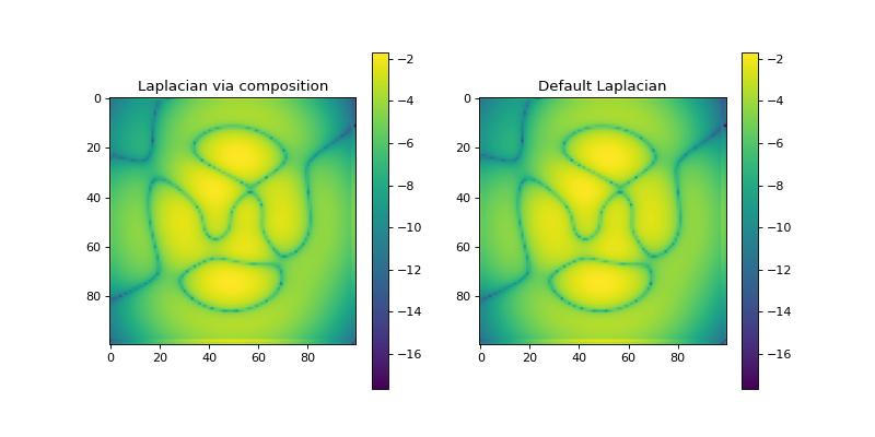
See also
- DirectionalGradient(dim_shape, directions, diff_method='fd', mode='constant', **diff_kwargs)[source]#
Directional gradient operator.
Notes
The
DirectionalGradientof a \(D\)-dimensional signal \(\mathbf{f} \in \mathbb{R}^{N_0 \times \cdots \times N_{D-1}}\) stacks the directional derivatives of \(\mathbf{f}\) along a list of \(m\) directions \(\mathbf{v}_i\) for \(1 \leq i \leq m\):\[\begin{split}\boldsymbol{\nabla}_{\mathbf{v}_1, \ldots ,\mathbf{v}_m} \mathbf{f} = \begin{bmatrix} \boldsymbol{\nabla}_{\mathbf{v}_1} \\ \vdots\\ \boldsymbol{\nabla}_{\mathbf{v}_m}\\ \end{bmatrix} \mathbf{f} \in \mathbb{R}^{m \times N_0 \times \cdots \times N_{D-1}},\end{split}\]where \(\boldsymbol{\nabla}_{\mathbf{v}_i}\) is the first-order directional derivative along \(\mathbf{v}_i\) implemented with
DirectionalDerivative(), with \(\mathbf{v}_i \in \mathbb{R}^D\) or \(\mathbf{v}_i \in \mathbb{R}^{D \times N_0 \times \cdots \times N_{D-1}}\).Note that choosing \(m=D\) and \(\mathbf{v}_i = \mathbf{e}_i \in \mathbb{R}^D\) (the \(i\)-th canonical basis vector) amounts to the
Gradient()operator.- Parameters:
dim_shape (
NDArrayShape) – Shape of the input array.directions (
list[NDArray]) – List of directions, either constant (array of size \((D,)\)) or spatially-varying (array of size \((D, N_0, \ldots, N_{D-1})\))diff_method (
"gd","fd") –Method used to approximate the derivative. Must be one of:
’fd’ (default): finite differences
’gd’: Gaussian derivative
mode (
str,list[str]) –Boundary conditions. Multiple forms are accepted:
str: unique mode shared amongst dimensions. Must be one of:
’constant’ (default): zero-padding
’wrap’
’reflect’
’symmetric’
’edge’
tuple[str, …]: the
d-th dimension usesmode[d]as boundary condition.
(See
numpy.pad()for details.)diff_kwargs (
dict) – Keyword arguments to parametrize partial derivatives (seefinite_difference()andgaussian_derivative())
- Returns:
op – Directional gradient
- Return type:
Example
import numpy as np
import matplotlib.pyplot as plt
from pyxu.operator import DirectionalGradient
from pyxu.util.misc import peaks

x = np.linspace(-2.5, 2.5, 25)
xx, yy = np.meshgrid(x, x)
z = peaks(xx, yy)
directions1 = np.zeros(shape=(2, z.size))
directions1[0, :z.size // 2] = 1
directions1[1, z.size // 2:] = 1
directions2 = np.zeros(shape=(2, z.size))
directions2[1, :z.size // 2] = -1
directions2[0, z.size // 2:] = -1
dim_shape = z.shape
dop = DirectionalGradient(dim_shape=dim_shape, directions=[directions1, directions2])
out = dop(z)
plt.figure()
h = plt.pcolormesh(xx, yy, z, shading='auto')
plt.quiver(x, x, directions1[1].reshape(dim_shape), directions1[0].reshape(xx.shape))
plt.quiver(x, x, directions2[1].reshape(dim_shape), directions2[0].reshape(xx.shape), color='red')
plt.colorbar(h)
plt.title(r'Signal $\mathbf{f}$ and directions of derivatives')
plt.figure()
h = plt.pcolormesh(xx, yy, out[0], shading='auto')
plt.colorbar(h)
plt.title(r'$\nabla_{\mathbf{v}_0} \mathbf{f}$')
plt.figure()
h = plt.pcolormesh(xx, yy, out[1], shading='auto')
plt.colorbar(h)
plt.title(r'$\nabla_{\mathbf{v}_1} \mathbf{f}$')


See also
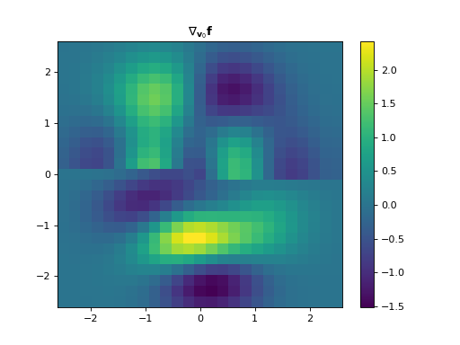
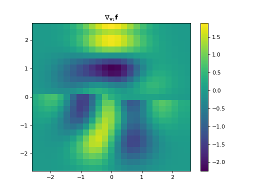
- DirectionalLaplacian(dim_shape, directions, weights=None, diff_method='fd', mode='constant', **diff_kwargs)[source]#
Directional Laplacian operator.
Sum of the second directional derivatives of a multi-dimensional array (at least two dimensions are required) along multiple
directionsfor each entry of the array.Notes
The
DirectionalLaplacianof a \(D\)-dimensional signal \(\mathbf{f} \in \mathbb{R}^{N_0 \times \cdots \times N_{D-1}}\) sums the second-order directional derivatives of \(\mathbf{f}\) along a list of \(m\) directions \(\mathbf{v}_i\) for \(1 \leq i \leq m\):\[\boldsymbol{\Delta}_{\mathbf{v}_1, \ldots ,\mathbf{v}_m} \mathbf{f} = \sum_{i=1}^m \boldsymbol{\nabla}^2_{\mathbf{v}_i} \mathbf{f} \in \mathbb{R}^{N_0 \times \cdots \times N_{D-1}},\]where \(\boldsymbol{\nabla}^2_{\mathbf{v}_i}\) is the second-order directional derivative along \(\mathbf{v}_i\) implemented with
DirectionalDerivative().Note that choosing \(m=D\) and \(\mathbf{v}_i = \mathbf{e}_i \in \mathbb{R}^D\) (the \(i\)-th canonical basis vector) amounts to the
Laplacian()operator.- Parameters:
dim_shape (
NDArrayShape) – Shape of the input array.directions (
list[NDArray]) – List of directions, either constant (array of size \((D,)\)) or spatially-varying (array of size \((D, N_0, \ldots, N_{D-1})\))weights (
list[Real],None) – List of optional positive weights with which each second directional derivative operator is multiplied.diff_method (
"gd","fd") –Method used to approximate the derivative. Must be one of:
’fd’ (default): finite differences
’gd’: Gaussian derivative
mode (
str,list[str]) –Boundary conditions. Multiple forms are accepted:
str: unique mode shared amongst dimensions. Must be one of:
’constant’ (default): zero-padding
’wrap’
’reflect’
’symmetric’
’edge’
tuple[str, …]: the
d-th dimension usesmode[d]as boundary condition.
(See
numpy.pad()for details.)diff_kwargs (
dict) – Keyword arguments to parametrize partial derivatives (seefinite_difference()andgaussian_derivative())
- Returns:
op – Directional Laplacian
- Return type:
Example
import numpy as np
import matplotlib.pyplot as plt
from pyxu.operator import DirectionalLaplacian
from pyxu.util.misc import peaks

x = np.linspace(-2.5, 2.5, 25)
xx, yy = np.meshgrid(x, x)
z = peaks(xx, yy)
directions1 = np.zeros(shape=(2, z.size))
directions1[0, :z.size // 2] = 1
directions1[1, z.size // 2:] = 1
directions2 = np.zeros(shape=(2, z.size))
directions2[1, :z.size // 2] = -1
directions2[0, z.size // 2:] = -1
dim_shape = z.shape
dop = DirectionalLaplacian(dim_shape=dim_shape, directions=[directions1, directions2])
out = dop(z)
plt.figure()
h = plt.pcolormesh(xx, yy, z, shading='auto')
plt.quiver(x, x, directions1[1].reshape(dim_shape), directions1[0].reshape(xx.shape))
plt.quiver(x, x, directions2[1].reshape(dim_shape), directions2[0].reshape(xx.shape), color='red')
plt.colorbar(h)
plt.title('Signal and directions of derivatives')
plt.figure()
h = plt.pcolormesh(xx, yy, out.squeeze(), shading='auto')
plt.colorbar(h)
plt.title('Directional Laplacian')


See also
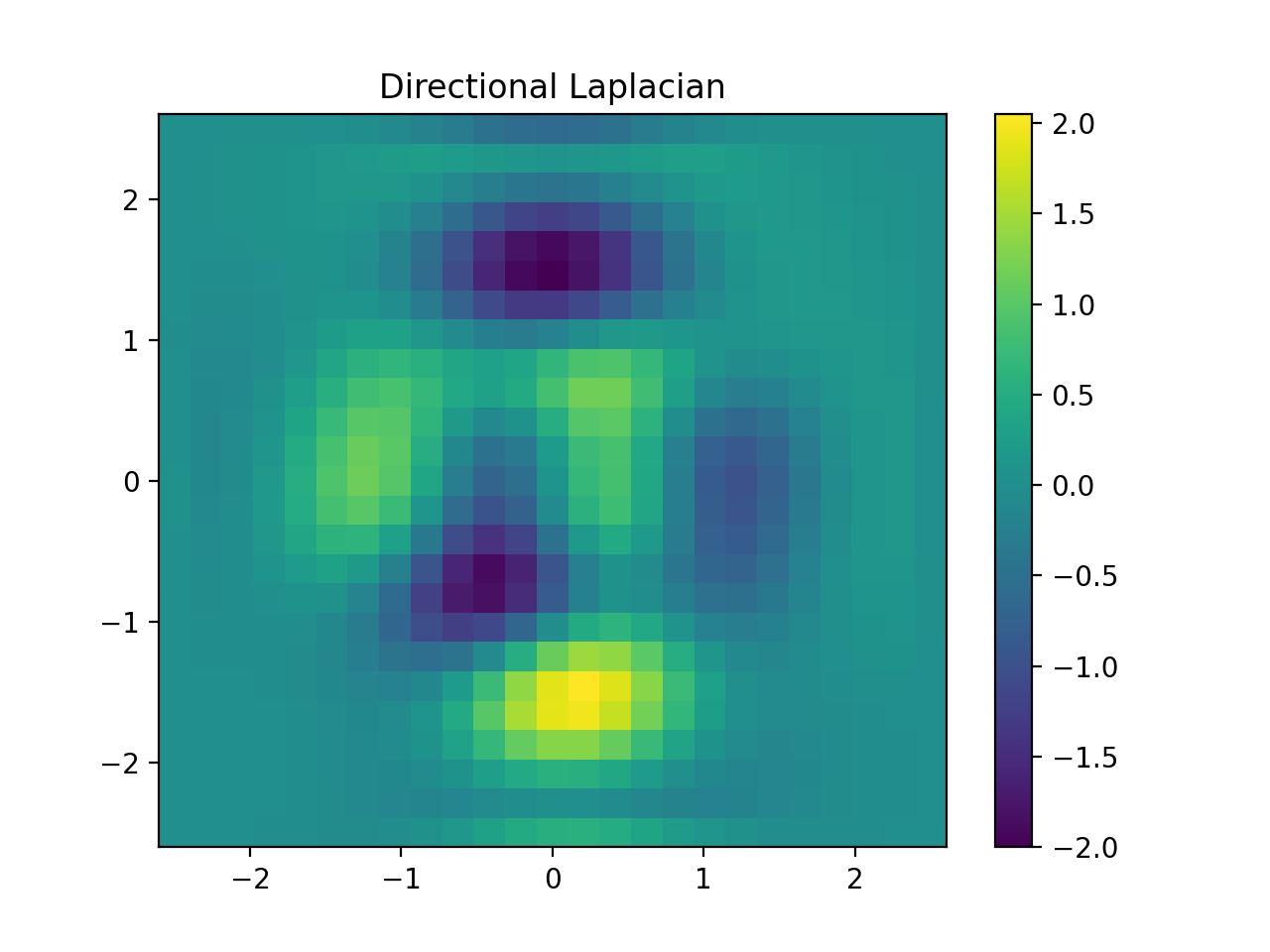
- DirectionalHessian(dim_shape, directions, diff_method='gd', mode='constant', **diff_kwargs)[source]#
Directional Hessian operator.
Notes
The
DirectionalHessianof a \(D\)-dimensional signal \(\mathbf{f} \in \mathbb{R}^{N_0 \times \cdots \times N_{D-1}}\) stacks the second-order directional derivatives of \(\mathbf{f}\) along a list of \(m\) directions \(\mathbf{v}_i\) for \(1 \leq i \leq m\):\[\begin{split}\mathbf{H}_{\mathbf{v}_1, \ldots ,\mathbf{v}_m} \mathbf{f} = \begin{bmatrix} \boldsymbol{\nabla}^2_{\mathbf{v}_0} & \cdots & \boldsymbol{\nabla}_{\mathbf{v}_0} \boldsymbol{\nabla}_{\mathbf{v}_{m-1}} \\ \vdots & \ddots & \vdots \\ \boldsymbol{\nabla}_{\mathbf{v}_{m-1}} \boldsymbol{\nabla}_{\mathbf{v}_0} & \cdots & \boldsymbol{\nabla}^2_{\mathbf{v}_{m-1}} \end{bmatrix} \mathbf{f},\end{split}\]where \(\boldsymbol{\nabla}_{\mathbf{v}_i}\) is the first-order directional derivative along \(\mathbf{v}_i\) implemented with
DirectionalDerivative().However, due to the symmetry of the Hessian, only the upper triangular part is computed in practice:
\[\begin{split}\mathbf{H}_{\mathbf{v}_1, \ldots ,\mathbf{v}_m} \mathbf{f} = \begin{bmatrix} \boldsymbol{\nabla}^2_{\mathbf{v}_0}\\ \boldsymbol{\nabla}_{\mathbf{v}_0} \boldsymbol{\nabla}_{\mathbf{v}_{1}} \\ \vdots \\ \boldsymbol{\nabla}^2_{\mathbf{v}_{m-1}} \end{bmatrix} \mathbf{f} \in \mathbb{R}^{\frac{m (m-1)}{2} \times N_0 \times \cdots \times N_{D-1}}\end{split}\]Note that choosing \(m=D\) and \(\mathbf{v}_i = \mathbf{e}_i \in \mathbb{R}^D\) (the \(i\)-th canonical basis vector) amounts to the
Hessian()operator.- Parameters:
dim_shape (
NDArrayShape) – Shape of the input array.directions (
list[NDArray]) – List of directions, either constant (array of size \((D,)\)) or spatially-varying (array of size \((D, N_0, \ldots, N_{D-1})\))diff_method (
"gd","fd") –Method used to approximate the derivative. Must be one of:
’fd’ (default): finite differences
’gd’: Gaussian derivative
mode (
str,list[str]) –Boundary conditions. Multiple forms are accepted:
str: unique mode shared amongst dimensions. Must be one of:
’constant’ (default): zero-padding
’wrap’
’reflect’
’symmetric’
’edge’
tuple[str, …]: the
d-th dimension usesmode[d]as boundary condition.
(See
numpy.pad()for details.)diff_kwargs (
dict) – Keyword arguments to parametrize partial derivatives (seefinite_difference()andgaussian_derivative())
- Returns:
op – Directional Hessian
- Return type:
Example
import numpy as np
import matplotlib.pyplot as plt
from pyxu.operator import DirectionalHessian
from pyxu.util.misc import peaks

x = np.linspace(-2.5, 2.5, 25)
xx, yy = np.meshgrid(x, x)
z = peaks(xx, yy)
directions1 = np.zeros(shape=(2, z.size))
directions1[0, :z.size // 2] = 1
directions1[1, z.size // 2:] = 1
directions2 = np.zeros(shape=(2, z.size))
directions2[1, :z.size // 2] = -1
directions2[0, z.size // 2:] = -1
dim_shape = z.shape
d_hess = DirectionalHessian(dim_shape=dim_shape, directions=[directions1, directions2])
out = d_hess(z)
plt.figure()
h = plt.pcolormesh(xx, yy, z, shading='auto')
plt.quiver(x, x, directions1[1].reshape(dim_shape), directions1[0].reshape(xx.shape))
plt.quiver(x, x, directions2[1].reshape(dim_shape), directions2[0].reshape(xx.shape), color='red')
plt.colorbar(h)
plt.title(r'Signal $\mathbf{f}$ and directions of derivatives')
plt.figure()
h = plt.pcolormesh(xx, yy, out[0], shading='auto')
plt.colorbar(h)
plt.title(r'$\nabla^2_{\mathbf{v}_0} \mathbf{f}$')
plt.figure()
h = plt.pcolormesh(xx, yy, out[1], shading='auto')
plt.colorbar(h)
plt.title(r'$\nabla_{\mathbf{v}_0} \nabla_{\mathbf{v}_{1}} \mathbf{f}$')
plt.figure()
h = plt.pcolormesh(xx, yy, out[2], shading='auto')
plt.colorbar(h)
plt.title(r'$\nabla^2_{\mathbf{v}_1} \mathbf{f}$')


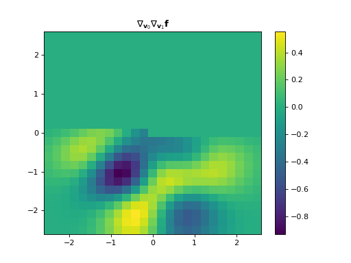
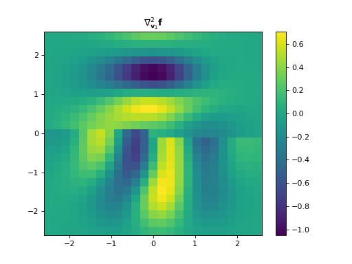
See also
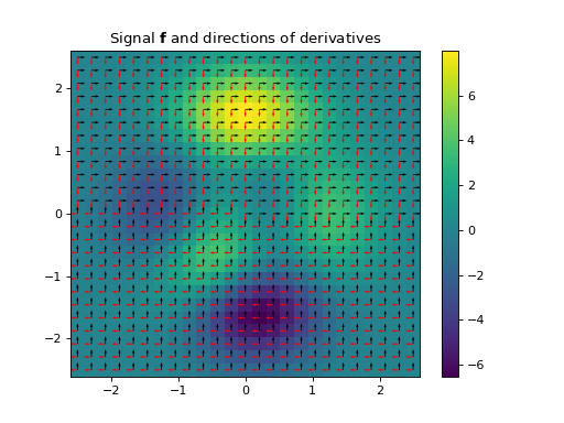
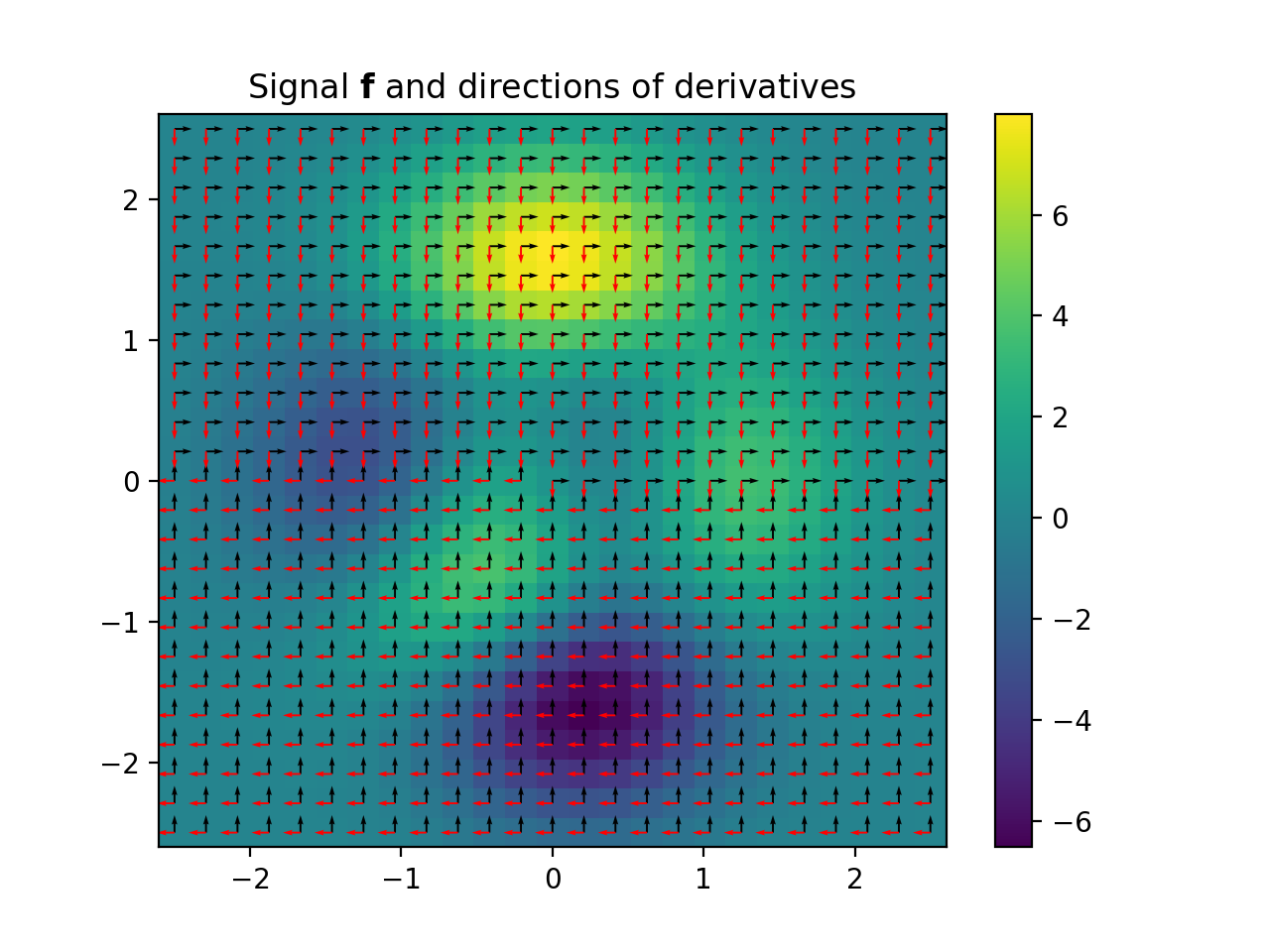
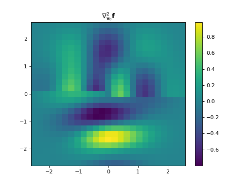
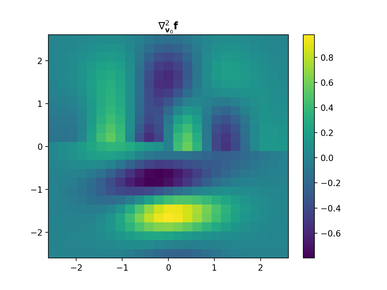
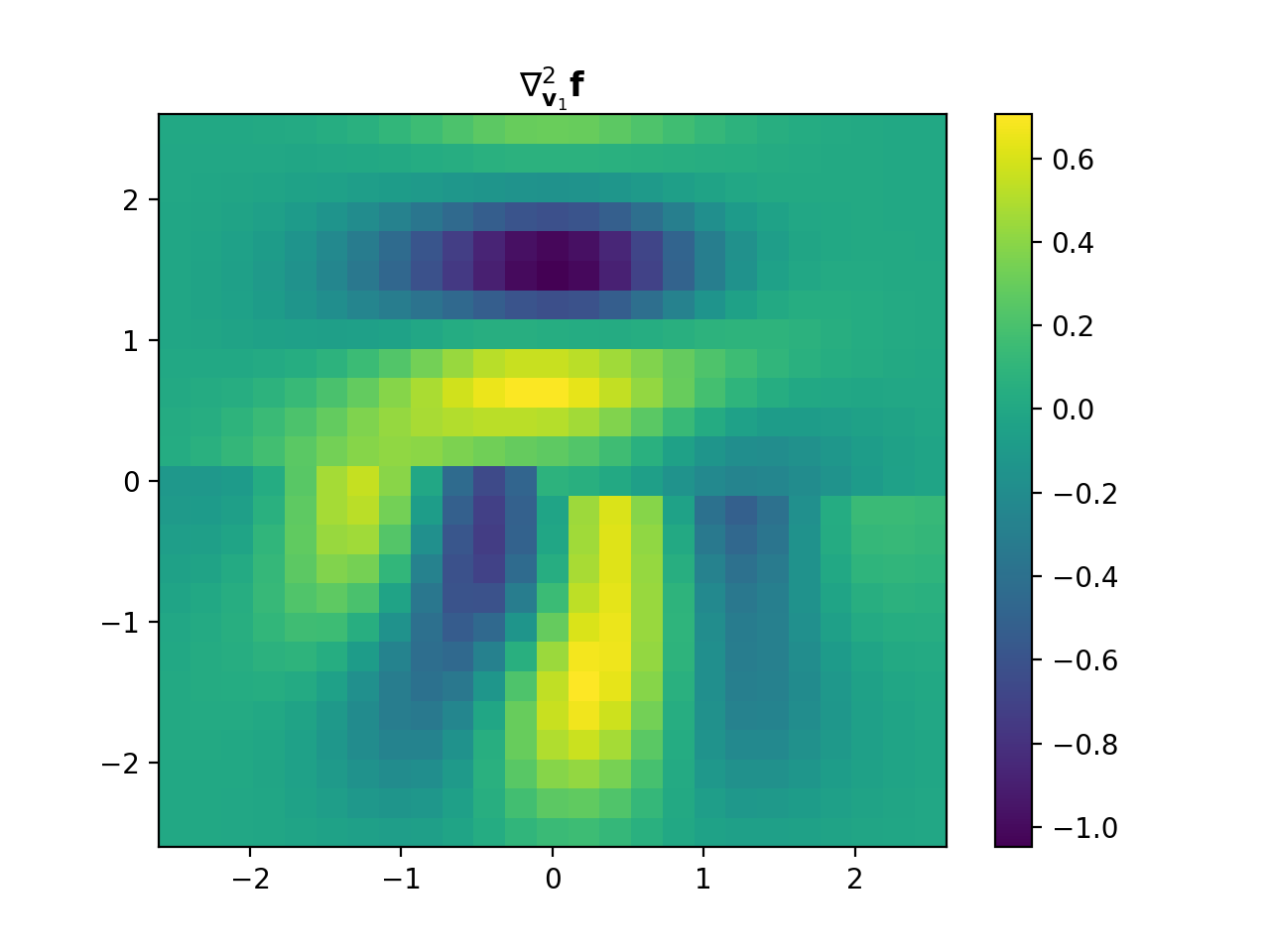
Tensor Products#
- kron(A, B)[source]#
Kronecker product \(A \otimes B\) between two linear operators.
The Kronecker product \(A \otimes B\) is defined as
\[\begin{split}A \otimes B = \left[ \begin{array}{ccc} A_{11} B & \cdots & A_{1N_{A}} B \\ \vdots & \ddots & \vdots \\ A_{M_{A}1} B & \cdots & A_{M_{A}N_{A}} B \\ \end{array} \right],\end{split}\]where \(A : \mathbb{R}^{N_{A}} \to \mathbb{R}^{M_{A}}\), and \(B : \mathbb{R}^{N_{B}} \to \mathbb{R}^{M_{B}}\).
- Parameters:
- Returns:
op – (mA*mB, nA*nB) linear operator.
- Return type:
Notes
This implementation is matrix-free by leveraging properties of the Kronecker product, i.e. \(A\) and \(B\) need not be known explicitly. In particular \((A \otimes B) x\) and \((A \otimes B)^{*} x\) are computed implicitly via the relation:
\[\text{vec}(\mathbf{A}\mathbf{B}\mathbf{C}) = (\mathbf{C}^{T} \otimes \mathbf{A}) \text{vec}(\mathbf{B}),\]where \(\mathbf{A}\), \(\mathbf{B}\), and \(\mathbf{C}\) are matrices.
- khatri_rao(A, B)[source]#
Column-wise Khatri-Rao product \(A \circ B\) between two linear operators.
The Khatri-Rao product \(A \circ B\) is defined as
\[A \circ B = \left[ \begin{array}{ccc} \mathbf{a}_{1} \otimes \mathbf{b}_{1} & \cdots & \mathbf{a}_{N} \otimes \mathbf{b}_{N} \end{array} \right],\]where \(A : \mathbb{R}^{N} \to \mathbb{R}^{M_{A}}\), \(B : \mathbb{R}^{N} \to \mathbb{R}^{M_{B}}\), and \(\mathbf{a}_{k}\) (repectively \(\mathbf{b}_{k}\)) denotes the \(k\)-th column of \(A\) (respectively \(B\)).
- Parameters:
- Returns:
op – (mA*mB, n) linear operator.
- Return type:
Notes
This implementation is matrix-free by leveraging properties of the Khatri-Rao product, i.e. \(A\) and \(B\) need not be known explicitly. In particular \((A \circ B) x\) and \((A \circ B)^{*} x\) are computed implicitly via the relation:
\[\text{vec}(\mathbf{A}\text{diag}(\mathbf{b})\mathbf{C}) = (\mathbf{C}^{T} \circ \mathbf{A}) \mathbf{b},\]where \(\mathbf{A}\), \(\mathbf{C}\) are matrices, and \(\mathbf{b}\) is a vector.
Note however that a matrix-free implementation of the Khatri-Rao product does not permit the same optimizations as a matrix-based implementation. Thus the Khatri-Rao product as implemented here is only marginally more efficient than applying
kron()and pruning its output.