pyxu.experimental.sampler

class MYULA(f=None, g=None, gamma=None, lamb=None)

Bases: ULA

Moreau-Yosida unajusted Langevin algorithm (MYULA).

Generates samples from the distribution

\[p(\mathbf{x}) = \frac{\exp(-\mathcal{F}(\mathbf{x}) - \mathcal{G}(\mathbf{x}))}{\int_{\mathbb{R}^N} \exp(-\mathcal{F}(\tilde{\mathbf{x}}) - \mathcal{G}(\tilde{\mathbf{x}})) \mathrm{d} \tilde{\mathbf{x}} },\]

where \(\mathcal{F}: \mathbb{R}^N \to \mathbb{R}\) is convex and differentiable with \(\beta\)- Lipschitz continuous gradient, and \(\mathcal{G}: \mathbb{R}^N \to \mathbb{R}\) is proper, lower semi- continuous and convex with simple proximal operator.

Notes

MYULA is an extension of ULA to sample from distributions whose logarithm is nonsmooth. It consists in applying ULA to the differentiable functional \(\mathcal{U}^\lambda = \mathcal{F} + \mathcal{G}^\lambda\) for some \(\lambda > 0\), where

\[\mathcal{G}^\lambda (\mathbf{x}) = \inf_{\tilde{\mathbf{x}} \in \mathbb{R}^N} \frac{1}{2 \lambda} \Vert \tilde{\mathbf{x}} - \mathbf{x} \Vert_2^2 + \mathcal{G}(\tilde{\mathbf{x}})\]

is the Moreau-Yosida envelope of \(\mathcal{G}\) with parameter \(\lambda\). We then have

\[\nabla \mathcal{U}^\lambda (\mathbf{x}) = \nabla \mathcal{F}(\mathbf{x}) + \frac{1}{\lambda} (\mathbf{x} - \mathrm{prox}_{\lambda \mathcal{G}}(\mathbf{x})),\]

hence \(\nabla \mathcal{U}^\lambda\) is \((\beta + \frac{1}{\lambda})\)-Lipschitz continuous, where \(\beta\) is the Lipschitz constant of \(\nabla \mathcal{F}\). Note that the target distribution of the underlying ULA Markov chain is not exactly \(p(\mathbf{x})\), but the distribution

\[p^\lambda(\mathbf{x}) \propto \exp(-\mathcal{F}(\mathbf{x})-\mathcal{G}^\lambda(\mathbf{x})),\]

which introduces some additional bias on top of the bias of ULA related to the step size \(\gamma\) (see Notes of ULA documentation). MYULA is guaranteed to converges when \(\gamma \leq \frac{1}{\beta + \frac{1}{\lambda}}\), in which case it converges toward the stationary distribution \(p^\lambda_\gamma(\mathbf{x})\) that satisfies

\[\lim_{\gamma, \lambda \to 0} \Vert p^\lambda_\gamma - p \Vert_{\mathrm{TV}} = 0\]

(see [MYULA]). The parameter \(\lambda\) parameter is subject to a similar bias-variance tradeoff as \(\gamma\). It is recommended to set it in the order of \(\frac{1}{\beta}\), so that the contributions of \(\mathcal{F}\) and \(\mathcal{G}^\lambda\) to the Lipschitz constant of \(\nabla \mathcal{U}^\lambda\) is well balanced.

Parameters:

• f (DiffFunc)

• g (ProxFunc)

• gamma (Real)

• lamb (Real)

__init__(f=None, g=None, gamma=None, lamb=None)

Parameters:

• f (DiffFunc, None) – Differentiable functional.

• g (ProxFunc, None) – Proximable functional.

• gamma (Real) – Euler-Maruyama discretization step of the Langevin equation (see Notes of ULA documentation).

• lamb (Real) – Moreau-Yosida envelope parameter for g.

class OnlineCenteredMoment(order=2)

Bases: _OnlineStat

Pointwise online centered moment.

For \(d \geq 2\), the \(d\)-th order centered moment of the \(K\) samples \((\mathbf{x}_k)_{1 \leq k \leq K}\) is given by \(\boldsymbol{\mu}_d=\frac{1}{K} \sum_{k=1}^K (\mathbf{x}_k-\boldsymbol{\mu})^d\), where \(\boldsymbol{\mu}\) is the sample mean.

Notes

This class implements the Welford algorithm described in [WelfordAlg], which is a numerically stable algorithm for computing online centered moments. In particular, it avoids catastrophic cancellation issues that may arise when naively computing online centered moments, which would lead to a loss of numerical precision.

Note that this class internally stores the values of all online centered moments of order \(d'\) for \(2 \leq d' \leq d\) in the attribute _corrected_sums as well as the online mean (_mean attribute). More precisely, the array _corrected_sums[i, :] corresponds to the online sum \(\boldsymbol{\mu}_{i+2}= \sum_{k=1}^K (\mathbf{x}_k-\boldsymbol{\mu})^{i+2}\) for \(0 \leq i \leq d-2\).

Parameters:

order (Real)

update(x)

Update the online statistic based on a new sample. Should update _num_samples and _stat attributes.

Parameters:

x (NDArray) – New sample.

Returns:

stat – Updated statistic.

Return type:

NDArray

OnlineKurtosis()

Pointwise online kurtosis.

The pointwise online variance of the \(K\) samples \((\mathbf{x}_k)_{1 \leq k \leq K}\) is given by \(\frac{1}{K}\sum_{k=1}^K \left( \frac{\mathbf{x}_k-\boldsymbol{\mu}}{\boldsymbol{\sigma}}\right)^4\), where \(\boldsymbol{\mu}\) is the sample mean and \(\boldsymbol{\sigma}\) its standard deviation.

Kurtosis is a measure of the heavy-tailedness of a distribution. In particular, the kurtosis of a Gaussian distribution is always 3.

class OnlineMoment(order=1)

Bases: _OnlineStat

Pointwise online moment.

For \(d \geq 1\), the \(d\)-th order centered moment of the \(K\) samples \((\mathbf{x}_k)_{1 \leq k \leq K}\) is given by \(\frac{1}{K}\sum_{k=1}^K \mathbf{x}_k^d\).

Parameters:

order (Real)

update(x)

Update the online statistic based on a new sample. Should update _num_samples and _stat attributes.

Parameters:

x (NDArray) – New sample.

Returns:

stat – Updated statistic.

Return type:

NDArray

OnlineSkewness()

Pointwise online skewness.

The pointwise online skewness of the \(K\) samples \((\mathbf{x}_k)_{1 \leq k \leq K}\) is given by \(\frac{1}{K}\sum_{k=1}^K \left( \frac{\mathbf{x}_k-\boldsymbol{\mu}}{\boldsymbol{\sigma}}\right)^3\), where \(\boldsymbol{\mu}\) is the sample mean and \(\boldsymbol{\sigma}\) its standard deviation.

Skewness is a measure of asymmetry of a distribution around its mean. Negative skewness indicates that the distribution has a heavier tail on the left side than on the right side, positive skewness indicates the opposite, and values close to zero indicate a symmetric distribution.

OnlineStd()

Pointwise online standard deviation.

The pointwise online standard deviation of the \(K\) samples \((\mathbf{x}_k)_{1 \leq k \leq K}\) is given by \(\boldsymbol{\sigma}=\sqrt{\frac{1}{K}\sum_{k=1}^K (\mathbf{x}_k - \boldsymbol{\mu})^2}\), where \(\boldsymbol{\mu}\) is the sample mean.

OnlineVariance()

Pointwise online variance.

The pointwise online variance of the \(K\) samples \((\mathbf{x}_k)_{1 \leq k \leq K}\) is given by \(\boldsymbol{\sigma}^2 = \frac{1}{K}\sum_{k=1}^K (\mathbf{x}_k-\boldsymbol{\mu})^2\), where \(\boldsymbol{\mu}\) is the sample mean.

class ULA(f, gamma=None)

Bases: _Sampler

Unajusted Langevin algorithm (ULA).

Generates samples from the distribution

\[p(\mathbf{x}) = \frac{\exp(-\mathcal{F}(\mathbf{x}))}{\int_{\mathbb{R}^N} \exp(-\mathcal{F}(\tilde{\mathbf{x}})) \mathrm{d} \tilde{\mathbf{x}} },\]

where \(\mathcal{F}: \mathbb{R}^N \to \mathbb{R}\) is differentiable with \(\beta\)-Lipschitz continuous gradient.

Notes

ULA is a Monte-Carlo Markov chain (MCMC) method that derives from the discretization of overdamped Langevin diffusions. More specifically, it relies on the Langevin stochastic differential equation (SDE):

\[\mathrm{d} \mathbf{X}_t = - \nabla \mathcal{F}(\mathbf{X}_t) \mathrm{d}t + \sqrt{2} \mathrm{d} \mathbf{B}_t,\]

where \((\mathbf{B}_t)_{t \geq 0}\) is a \(N\)-dimensional Brownian motion. It is well known that under mild technical assumptions, this SDE has a unique strong solution whose invariant distribution is \(p(\mathbf{x}) \propto \exp(-\mathcal{F}(\mathbf{x}))\). The discrete-time Euler-Maruyama discretization of this SDE then yields the ULA Markov chain

\[\mathbf{X}_{k+1} = \mathbf{X}_{k} - \gamma \nabla \mathcal{F}(\mathbf{X}_k) + \sqrt{2 \gamma} \mathbf{Z}_{k+1}\]

for all \(k \in \mathbb{Z}\), where \(\gamma\) is the discretization step size and \((\mathbf{Z}_k)_{k \in \mathbb{Z}}\) is a sequence of independant and identically distributed \(N\)-dimensional standard Gaussian distributions. When \(\mathcal{F}\) is differentiable with \(\beta\)-Lipschitz continuous gradient and \(\gamma \leq \frac{1}{\beta}\), the ULA Markov chain converges (see [ULA]) to a unique stationary distribution \(p_\gamma\) such that

\[\lim_{\gamma \to 0} \Vert p_\gamma - p \Vert_{\mathrm{TV}} = 0.\]

The discretization step \(\gamma\) is subject to the bias-variance tradeoff: a larger step will lead to faster convergence of the Markov chain at the expense of a larger bias in the approximation of the distribution \(p\). Setting \(\gamma\) as large as possible (default behavior) is recommended for large-scale problems, since convergence speed (rather than approximation bias) is then typically the main bottelneck. See Example section below for a concrete illustration of this tradeoff.

Remarks

Like all MCMC sampling methods, ULA comes with the following challenges:

• The first few samples of the chain may not be adequate for computing statistics, as they might be located in low probability regions. This challenge can either be alleviated by selecting a representative starting point to the chain, or by having a burn-in phase where the first few samples are discarded.

• Consecutive samples are typically correlated, which can deteriorate the Monte-Carlo estimation of quantities of interest. This issue can be alleviated by thinning the chain, i.e., selecting only every \(k\) samples, at the expense of an increased computational cost. Useful diagnostic tools to quantify this correlation between samples include the pixel-wise autocorrelation function and the effective sample size.

Example

We illustrate ULA on a 1D example (\(N = 1\)) where \(\mathcal{F}(x) = \frac{x^2}{2}\); the target distribution \(p(x)\) is thus the 1D standard Gaussian. In this toy example, the biased distribution \(p_\gamma(x)\) can be computed in closed form. The ULA Markov chain is given by

\[\begin{split}\mathbf{X}_{k+1} &= \mathbf{X}_{k} - \gamma \nabla\mathcal{F}(\mathbf{X}_k) + \sqrt{2\gamma}\mathbf{Z}_{k+1} \\ &= \mathbf{X}_{k} (1 - \gamma) + \sqrt{2 \gamma} \mathbf{Z}_{k+1}.\end{split}\]

Assuming for simplicity that \(\mathbf{X}_0\) is Gaussian with mean \(\mu_0\) and variance \(\sigma_0^2\), \(\mathbf{X}_k\) is Gaussian for any \(k \in \mathbb{Z}\) as a linear combination of Gaussians. Taking the expected value of the recurrence relation yields

\[\mu_k := \mathbb{E}(\mathbf{X}_{k}) = \mathbb{E}(\mathbf{X}_{k-1}) (1 - \gamma) = \mu_0 (1 - \gamma)^k\]

(geometric sequence). Taking the expected value of the square of the recurrence relation yields

\[\mu^{(2)}_k := \mathbb{E}(\mathbf{X}_{k}^2) = \mathbb{E}(\mathbf{X}_{k-1}^2) (1 - \gamma)^2 + 2 \gamma = (1 - \gamma)^{2k} (\sigma_0^2 - b) + b\]

with \(b = \frac{2 \gamma}{1 - (1 - \gamma)^{2}} = \frac{1}{1-\frac{\gamma}{2}}\) (arithmetico-geometric sequence) due to the independence of \(\mathbf{X}_{k-1}\) and \(\mathbf{Z}_{k}\). Hence, \(p_\gamma(x)\) is a Gaussian with mean \(\mu_\gamma= \lim_{k \to \infty} \mu_k = 0\) and variance \(\sigma_\gamma^2 = \lim_{k \to \infty} \mu^{(2)}_k - \mu_k^2 = \frac{1}{1-\frac{\gamma}{2}}\). As expected, we have \(\lim_{\gamma \to 0} \sigma_\gamma^2 = 1\), which is the variance of the target distribution \(p(x)\).

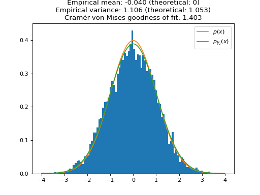
We plot the distribution of the samples of ULA for one large (\(\gamma_1 \approx 1\), i.e. \(\sigma_{\gamma_1}^2 \approx 2\)) and one small (\(\gamma_2 = 0.1\), i.e. \(\sigma_{\gamma_2}^2 \approx 1.05\)) step size. As expected, the larger step size \(\gamma_1\) leads to a larger bias in the approximation of \(p(x)\). To quantify the speed of convergence of the Markov chains, we compute the Cramér-von Mises tests of goodness of fit of the empirical distributions to the stationary distributions of ULA \(p_{\gamma_1}(x)\) and \(p_{\gamma_2}(x)\). We observe that the larger step \(\gamma_1\) leads to a better fit (lower Cramér-von Mises criterion), which illustrates the aforementioned bias-variance tradeoff for the choice of the step size.

import matplotlib.pyplot as plt
import numpy as np
import pyxu.experimental.sampler as pxe_sampler
import pyxu.operator as pxo
import scipy as sp

f = pxo.SquaredL2Norm(dim_shape=1) / 2  # To sample 1D normal distribution (mean 0, variance 1)
ula = pxe_sampler.ULA(f=f)  # Sampler with maximum step size
ula_lb = pxe_sampler.ULA(f=f, gamma=1e-1)  # Sampler with small step size

gen_ula = ula.samples(x0=np.zeros(1))
gen_ula_lb = ula_lb.samples(x0=np.zeros(1))
n_burn_in = int(1e3)  # Number of burn-in iterations
for i in range(n_burn_in):
    next(gen_ula)
    next(gen_ula_lb)

# Online statistics objects
mean_ula = pxe_sampler.OnlineMoment(order=1)
mean_ula_lb = pxe_sampler.OnlineMoment(order=1)
var_ula = pxe_sampler.OnlineVariance()
var_ula_lb = pxe_sampler.OnlineVariance()

n = int(1e4)  # Number of samples
samples_ula = np.zeros(n)
samples_ula_lb = np.zeros(n)
for i in range(n):
    sample = next(gen_ula)
    sample_lb = next(gen_ula_lb)
    samples_ula[i] = sample
    samples_ula_lb[i] = sample_lb
    mean = float(mean_ula.update(sample))
    var = float(var_ula.update(sample))
    mean_lb = float(mean_ula_lb.update(sample_lb))
    var_lb = float(var_ula_lb.update(sample_lb))

# Theoretical variances of biased stationary distributions of ULA
biased_var = 1 / (1 - ula._gamma / 2)
biased_var_lb = 1 / (1 - ula_lb._gamma / 2)

# Quantify goodness of fit of empirical distribution with theoretical distribution (Cramér-von Mises test)
cvm = sp.stats.cramervonmises(samples_ula, "norm", args=(0, np.sqrt(biased_var)))
cvm_lb = sp.stats.cramervonmises(samples_ula_lb, "norm", args=(0, np.sqrt(biased_var_lb)))

# Plots
grid = np.linspace(-4, 4, 1000)

plt.figure()
plt.title(
    f"ULA samples (large step size) \n Empirical mean: {mean:.3f} (theoretical: 0) \n "
    f"Empirical variance: {var:.3f} (theoretical: {biased_var:.3f}) \n"
    f"Cramér-von Mises goodness of fit: {cvm.statistic:.3f}"
)
plt.hist(samples_ula, range=(min(grid), max(grid)), bins=100, density=True)
plt.plot(grid, sp.stats.norm.pdf(grid), label=r"$p(x)$")
plt.plot(grid, sp.stats.norm.pdf(grid, scale=np.sqrt(biased_var)), label=r"$p_{\gamma_1}(x)$")
plt.legend()
plt.show()

(Source code, png, hires.png, pdf)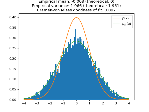

plt.figure()
plt.title(
    f"ULA samples (small step size) \n Empirical mean: {mean_lb:.3f} (theoretical: 0) \n "
    f"Empirical variance: {var_lb:.3f} (theoretical: {biased_var_lb:.3f}) \n"
    f"Cramér-von Mises goodness of fit: {cvm_lb.statistic:.3f}"
)
plt.hist(samples_ula_lb, range=(min(grid), max(grid)), bins=100, density=True)
plt.plot(grid, sp.stats.norm.pdf(grid), label=r"$p(x)$")
plt.plot(grid, sp.stats.norm.pdf(grid, scale=np.sqrt(biased_var_lb)), label=r"$p_{\gamma_2}(x)$")
plt.legend()
plt.show()

(png, hires.png, pdf)

__init__(f, gamma=None)

Parameters:

• f (DiffFunc) – Differentiable functional.

• gamma (Real) – Euler-Maruyama discretization step of the Langevin equation (see Notes).

objective_func()

Negative logarithm of the target ditribution (up to the a constant) evaluated at the current state of the Markov chain.

Useful for diagnostics purposes to monitor whether the Markov chain is sufficiently warm-started. If so, the samples should accumulate around the modes of the target distribution, i.e., toward the minimum of \(\mathcal{F}\).

Return type:

Real

Parameters:

• f (DiffFunc)

• gamma (Real)