[1]:
import numpy as np
import matplotlib.pyplot as plt
import skimage
from pyxu.operator import Convolve
Convolution with Pyxu#
0) Install dependencies#
You’ll need some additional dependencies to run this example:
tqdm (https://tqdm.github.io/)
Warning: this notebook benchmarks different packages and can take a few minutes to execute.
1) Prepare data#
Create input image#
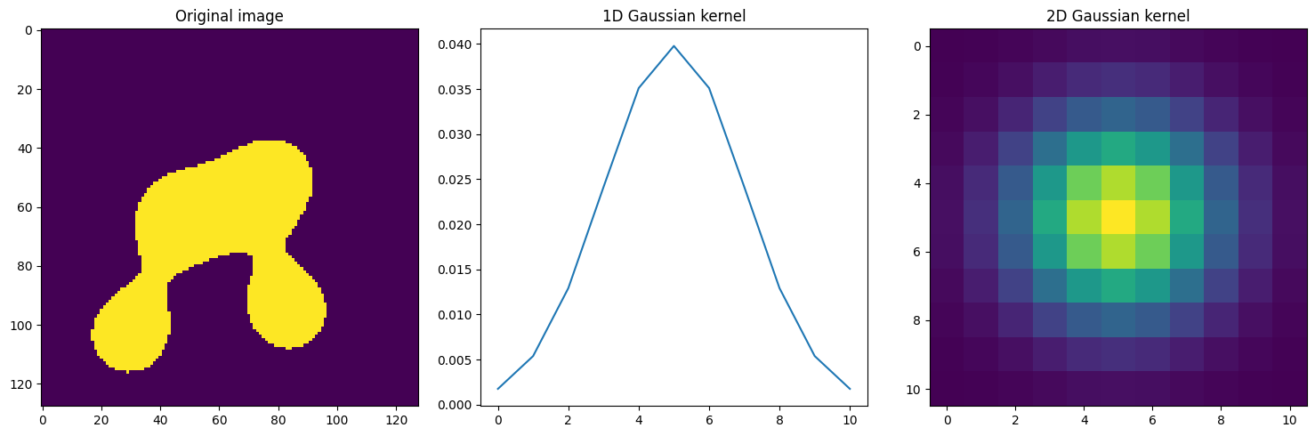
We first start creating a 2D binary image of size 128x128 with blobs, where the blobs occupy approximately 20% of the image’s area and are about half the size of the image.
The resulting binary image is then converted to a floating-point representation.
[2]:
npix = 128
data = skimage.data.binary_blobs(
    length=npix,
    blob_size_fraction=0.5,
    n_dim=2,
    volume_fraction=0.2,
).astype(float)
Create blurring kernel#
[3]:
sigma = 2  # Gaussian kernel std
width = 11  # Length of the Graussian kernel
gauss = lambda x: (1 / (2 * np.pi * sigma**2)) * np.exp(
    -0.5 * ((x - (width - 1) / 2) ** 2) / (sigma**2)
)
kernel_1d = np.fromfunction(gauss, (width,))
kernel_2d = np.outer(kernel_1d.reshape(-1, 1), kernel_1d.reshape(1, -1))
[4]:
fig, axs = plt.subplots(1, 3, figsize=(15, 5))

axs[0].imshow(data)
axs[0].set_title("Original image")

axs[1].plot(kernel_1d)
axs[1].set_title("1D Gaussian kernel")

axs[2].imshow(kernel_2d)
axs[2].set_title("2D Gaussian kernel")

fig.tight_layout();
2) Convolve image#
Scipy#
If you want to use scipy.signal.convolve() to perform 2D convolutions, it expects the kernel to match the dimensionality of the input data. So, for 2D data, you would generally provide a 2D kernel.
[5]:
from scipy.signal import convolve as conv_scipy

# Direct 2D convolution
y = conv_scipy(data, kernel_2d, mode="same", method="direct")
However, when dealing with a separable kernel (like a Gaussian kernel), you can take advantage of the kernel’s separability to perform convolution more efficiently:
First, convolve the input 2D data with the 1D kernel along one dimension (e.g., rows).
Then, convolve the result from the first step with the same 1D kernel along the other dimension (e.g., columns).
[6]:
# Separable convolution ...

convolved_rows = conv_scipy(  # ... along rows
    data,
    kernel_1d[:, np.newaxis],
    mode="same",
    method="direct",
)

y_separable = conv_scipy(  # ... then along columns
    convolved_rows,
    kernel_1d[np.newaxis, :],
    mode="same",
    method="direct",
)

assert np.allclose(y, y_separable)
Pyxu#
Pyxu is optimized to handle separable kernels, which enhances performance. When working with such kernels, Pyxu can directly manage the separable convolution. Additionally, Pyxu leverages Numba.stencil to just-in-time (JIT) compile the convolution under the hood to make it faster. Here’s how you can use it:
[7]:
conv = Convolve(
    dim_shape=data.shape,
    kernel=[kernel_1d, kernel_1d],
    center=[width // 2, width // 2],
    mode="constant",
    enable_warnings=True,
)
y_pyxu = conv(data)

assert np.allclose(y, y_pyxu)
PyLops#
PyLops uses a flattened (raveled) version of your 2D data when applying the linear operator, so you need to flatten and reshape your data as you move between operations. If you want to perform a separable convolution, you need to manually decompose the 2D kernel into two 1D kernels, then apply two separate 1D convolution operations sequentially. This adds an extra layer of complexity in the implementation compared to just using a 2D convolution directly.
[8]:
!pip install pylops
Collecting pylops
  Using cached pylops-2.2.0-py3-none-any.whl.metadata (18 kB)
Requirement already satisfied: numpy>=1.21.0 in /home/ruequera/miniconda3/envs/pyxu/lib/python3.11/site-packages (from pylops) (1.26.3)
Requirement already satisfied: scipy>=1.4.0 in /home/ruequera/miniconda3/envs/pyxu/lib/python3.11/site-packages (from pylops) (1.11.4)
Using cached pylops-2.2.0-py3-none-any.whl (287 kB)
Installing collected packages: pylops
Successfully installed pylops-2.2.0
[10]:
from pyxu.operator.interop import from_sciop
import pyxu.abc as pxa

from pylops.signalprocessing import Convolve2D

# 2d convolution
conv_pylops = from_sciop(
    cls=pxa.LinOp,
    sp_op=Convolve2D(
        dims=data.shape,
        h=kernel_2d,
        offset=np.r_[width // 2, width // 2],
        axes=(0, 1),
        method="direct",
    ),
)
y_pylops = conv_pylops(data.ravel()).reshape(data.shape)
assert np.allclose(y, y_pylops)
[11]:
# Separable convolution
conv_pylops_rows = from_sciop(
    cls=pxa.LinOp,
    sp_op=Convolve2D(
        dims=data.shape,
        h=kernel_1d[np.newaxis, :],
        offset=np.r_[0, width // 2],
        axes=(0, 1),
        method="direct",
    ),
)
conv_pylops_cols = from_sciop(
    cls=pxa.LinOp,
    sp_op=Convolve2D(
        dims=data.shape,
        h=kernel_1d[:, np.newaxis],
        offset=np.r_[width // 2, 0],
        axes=(0, 1),
        method="direct",
    ),
)

y_pylops = conv_pylops_cols(conv_pylops_rows(data.ravel())).reshape(data.shape)
assert np.allclose(y, y_pylops)
Scico#
Like Pyxu, Scico employs JIT (Just-In-Time) compilation to speed up convolution operations. However, Scico relies on Jax instead of Numba. This necessitates the transition of our array module from NumPy to Jax.
In a manner similar to PyLops, Scico expects the convolutional kernel to have the same dimensionality as the input image. One can opt for a more efficient combination of two 1D operators or a simpler single 2D operator.
[12]:
!pip install scico
Collecting scico
  Using cached scico-0.0.5.post1-py3-none-any.whl.metadata (3.8 kB)
Requirement already satisfied: typing-extensions in /home/ruequera/miniconda3/envs/pyxu/lib/python3.11/site-packages (from scico) (4.9.0)
Requirement already satisfied: numpy>=1.20.0 in /home/ruequera/miniconda3/envs/pyxu/lib/python3.11/site-packages (from scico) (1.26.3)
Requirement already satisfied: scipy>=1.6.0 in /home/ruequera/miniconda3/envs/pyxu/lib/python3.11/site-packages (from scico) (1.11.4)
Requirement already satisfied: imageio>=2.17 in /home/ruequera/miniconda3/envs/pyxu/lib/python3.11/site-packages (from scico) (2.33.1)
Requirement already satisfied: matplotlib in /home/ruequera/miniconda3/envs/pyxu/lib/python3.11/site-packages (from scico) (3.8.2)
Collecting jaxlib<=0.4.23,>=0.4.3 (from scico)
  Using cached jaxlib-0.4.23-cp311-cp311-manylinux2014_x86_64.whl.metadata (2.1 kB)
Collecting jax<=0.4.23,>=0.4.3 (from scico)
  Using cached jax-0.4.23-py3-none-any.whl.metadata (24 kB)
Collecting orbax-checkpoint (from scico)
  Using cached orbax_checkpoint-0.5.0-py3-none-any.whl.metadata (1.7 kB)
Collecting flax<=0.7.5,>=0.6.1 (from scico)
  Using cached flax-0.7.5-py3-none-any.whl.metadata (10 kB)
Collecting pyabel>=0.9.0 (from scico)
  Using cached PyAbel-0.9.0-py3-none-any.whl
Requirement already satisfied: msgpack in /home/ruequera/miniconda3/envs/pyxu/lib/python3.11/site-packages (from flax<=0.7.5,>=0.6.1->scico) (1.0.7)
Collecting optax (from flax<=0.7.5,>=0.6.1->scico)
  Using cached optax-0.1.8-py3-none-any.whl.metadata (14 kB)
Collecting tensorstore (from flax<=0.7.5,>=0.6.1->scico)
  Using cached tensorstore-0.1.52-cp311-cp311-manylinux_2_17_x86_64.manylinux2014_x86_64.whl.metadata (3.0 kB)
Requirement already satisfied: rich>=11.1 in /home/ruequera/miniconda3/envs/pyxu/lib/python3.11/site-packages (from flax<=0.7.5,>=0.6.1->scico) (13.7.0)
Requirement already satisfied: PyYAML>=5.4.1 in /home/ruequera/miniconda3/envs/pyxu/lib/python3.11/site-packages (from flax<=0.7.5,>=0.6.1->scico) (6.0.1)
Requirement already satisfied: pillow>=8.3.2 in /home/ruequera/miniconda3/envs/pyxu/lib/python3.11/site-packages (from imageio>=2.17->scico) (10.2.0)
Collecting ml-dtypes>=0.2.0 (from jax<=0.4.23,>=0.4.3->scico)
  Using cached ml_dtypes-0.3.2-cp311-cp311-manylinux_2_17_x86_64.manylinux2014_x86_64.whl.metadata (20 kB)
Collecting opt-einsum (from jax<=0.4.23,>=0.4.3->scico)
  Using cached opt_einsum-3.3.0-py3-none-any.whl (65 kB)
Requirement already satisfied: setuptools>=44.0 in /home/ruequera/miniconda3/envs/pyxu/lib/python3.11/site-packages (from pyabel>=0.9.0->scico) (68.2.2)
Requirement already satisfied: six>=1.10.0 in /home/ruequera/miniconda3/envs/pyxu/lib/python3.11/site-packages (from pyabel>=0.9.0->scico) (1.16.0)
Requirement already satisfied: contourpy>=1.0.1 in /home/ruequera/miniconda3/envs/pyxu/lib/python3.11/site-packages (from matplotlib->scico) (1.2.0)
Requirement already satisfied: cycler>=0.10 in /home/ruequera/miniconda3/envs/pyxu/lib/python3.11/site-packages (from matplotlib->scico) (0.12.1)
Requirement already satisfied: fonttools>=4.22.0 in /home/ruequera/miniconda3/envs/pyxu/lib/python3.11/site-packages (from matplotlib->scico) (4.47.2)
Requirement already satisfied: kiwisolver>=1.3.1 in /home/ruequera/miniconda3/envs/pyxu/lib/python3.11/site-packages (from matplotlib->scico) (1.4.5)
Requirement already satisfied: packaging>=20.0 in /home/ruequera/miniconda3/envs/pyxu/lib/python3.11/site-packages (from matplotlib->scico) (23.2)
Requirement already satisfied: pyparsing>=2.3.1 in /home/ruequera/miniconda3/envs/pyxu/lib/python3.11/site-packages (from matplotlib->scico) (3.1.1)
Requirement already satisfied: python-dateutil>=2.7 in /home/ruequera/miniconda3/envs/pyxu/lib/python3.11/site-packages (from matplotlib->scico) (2.8.2)
Collecting absl-py (from orbax-checkpoint->scico)
  Using cached absl_py-2.1.0-py3-none-any.whl.metadata (2.3 kB)
Collecting etils[epath,epy] (from orbax-checkpoint->scico)
  Using cached etils-1.6.0-py3-none-any.whl.metadata (6.4 kB)
Requirement already satisfied: nest_asyncio in /home/ruequera/miniconda3/envs/pyxu/lib/python3.11/site-packages (from orbax-checkpoint->scico) (1.5.8)
Collecting protobuf (from orbax-checkpoint->scico)
  Using cached protobuf-4.25.2-cp37-abi3-manylinux2014_x86_64.whl.metadata (541 bytes)
Requirement already satisfied: markdown-it-py>=2.2.0 in /home/ruequera/miniconda3/envs/pyxu/lib/python3.11/site-packages (from rich>=11.1->flax<=0.7.5,>=0.6.1->scico) (3.0.0)
Requirement already satisfied: pygments<3.0.0,>=2.13.0 in /home/ruequera/miniconda3/envs/pyxu/lib/python3.11/site-packages (from rich>=11.1->flax<=0.7.5,>=0.6.1->scico) (2.17.2)
Requirement already satisfied: fsspec in /home/ruequera/miniconda3/envs/pyxu/lib/python3.11/site-packages (from etils[epath,epy]->orbax-checkpoint->scico) (2023.12.2)
Collecting importlib_resources (from etils[epath,epy]->orbax-checkpoint->scico)
  Using cached importlib_resources-6.1.1-py3-none-any.whl.metadata (4.1 kB)
Requirement already satisfied: zipp in /home/ruequera/miniconda3/envs/pyxu/lib/python3.11/site-packages (from etils[epath,epy]->orbax-checkpoint->scico) (3.17.0)
Collecting chex>=0.1.7 (from optax->flax<=0.7.5,>=0.6.1->scico)
  Using cached chex-0.1.85-py3-none-any.whl.metadata (17 kB)
Requirement already satisfied: toolz>=0.9.0 in /home/ruequera/miniconda3/envs/pyxu/lib/python3.11/site-packages (from chex>=0.1.7->optax->flax<=0.7.5,>=0.6.1->scico) (0.12.0)
Requirement already satisfied: mdurl~=0.1 in /home/ruequera/miniconda3/envs/pyxu/lib/python3.11/site-packages (from markdown-it-py>=2.2.0->rich>=11.1->flax<=0.7.5,>=0.6.1->scico) (0.1.2)
Using cached scico-0.0.5.post1-py3-none-any.whl (11.3 MB)
Using cached flax-0.7.5-py3-none-any.whl (244 kB)
Using cached jax-0.4.23-py3-none-any.whl (1.7 MB)
Using cached jaxlib-0.4.23-cp311-cp311-manylinux2014_x86_64.whl (77.2 MB)
Using cached orbax_checkpoint-0.5.0-py3-none-any.whl (136 kB)
Using cached ml_dtypes-0.3.2-cp311-cp311-manylinux_2_17_x86_64.manylinux2014_x86_64.whl (2.2 MB)
Using cached tensorstore-0.1.52-cp311-cp311-manylinux_2_17_x86_64.manylinux2014_x86_64.whl (14.1 MB)
Using cached absl_py-2.1.0-py3-none-any.whl (133 kB)
Using cached optax-0.1.8-py3-none-any.whl (199 kB)
Using cached protobuf-4.25.2-cp37-abi3-manylinux2014_x86_64.whl (294 kB)
Using cached chex-0.1.85-py3-none-any.whl (95 kB)
Using cached etils-1.6.0-py3-none-any.whl (144 kB)
Using cached importlib_resources-6.1.1-py3-none-any.whl (33 kB)
Installing collected packages: protobuf, opt-einsum, ml-dtypes, importlib_resources, etils, absl-py, tensorstore, pyabel, jaxlib, jax, chex, orbax-checkpoint, optax, flax, scico
Successfully installed absl-py-2.1.0 chex-0.1.85 etils-1.6.0 flax-0.7.5 importlib_resources-6.1.1 jax-0.4.23 jaxlib-0.4.23 ml-dtypes-0.3.2 opt-einsum-3.3.0 optax-0.1.8 orbax-checkpoint-0.5.0 protobuf-4.25.2 pyabel-0.9.0 scico-0.0.5.post1 tensorstore-0.1.52
[13]:
from scico.linop import Convolve as Conv_scico
from jax import config
import jax.numpy as jnp

# Convert data and kernel from Numpy to Jax
data_jax = jnp.asarray(data)
k2d_jax = jnp.asarray(kernel_2d)
config.update("jax_enable_x64", True)

# 2d convolution
conv_scico = Conv_scico(
    k2d_jax,
    input_shape=data_jax.shape,
    input_dtype=data_jax.dtype,
    mode="same",
    jit=True,
)
y_scico = conv_scico(data_jax)
assert np.allclose(y, y_scico)
[14]:
# Separable convolution
k1d_jax = jnp.asarray(kernel_1d)

conv_scico_rows = Conv_scico(
    k1d_jax[np.newaxis, :],
    input_shape=data_jax.shape,
    input_dtype=data_jax.dtype,
    mode="same",
    jit=True,
)
conv_scico_cols = Conv_scico(
    k1d_jax[:, np.newaxis],
    input_shape=data_jax.shape,
    input_dtype=data_jax.dtype,
    mode="same",
    jit=True,
)
y_scico = conv_scico_cols(conv_scico_rows(data_jax))
assert np.allclose(y, y_scico)
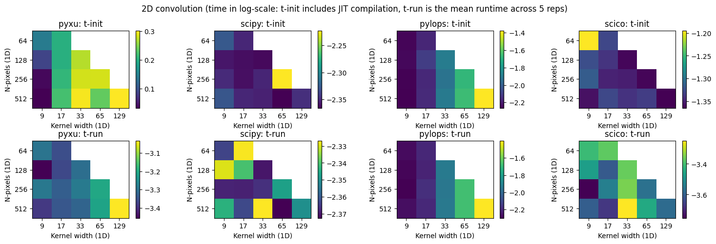
3) Benchmark convolution runtime across all libraries#
Separable 1d convolution#
[15]:
!pip install tqdm
Collecting tqdm
  Using cached tqdm-4.66.1-py3-none-any.whl.metadata (57 kB)
Using cached tqdm-4.66.1-py3-none-any.whl (78 kB)
Installing collected packages: tqdm
Successfully installed tqdm-4.66.1
[17]:
import time
import tqdm

npixs = [2**i for i in range(6, 10)]
nwidths = [2**i + 1 for i in range(3, 8)]

t_pyxu = np.full((2, len(npixs), len(nwidths)), np.nan)
t_scipy = np.full((2, len(npixs), len(nwidths)), np.nan)
t_pylops = np.full((2, len(npixs), len(nwidths)), np.nan)
t_scico = np.full((2, len(npixs), len(nwidths)), np.nan)

sigma = 2
gauss = lambda x: (1 / (2 * np.pi * sigma**2)) * np.exp(
    -0.5 * ((x - (width - 1) / 2) ** 2) / (sigma**2)
)

nreps = 5

with tqdm.tqdm(total=len(npixs) * len(nwidths)) as pbar:
    for i, npix in enumerate(npixs):
        x = skimage.data.binary_blobs(
            length=npix, blob_size_fraction=0.5, n_dim=2, volume_fraction=0.2
        ).astype(float)
        for j, width in enumerate(nwidths):
            if npix > (width * 2):
                kernel = np.fromfunction(gauss, (width,))
                data_jax = jnp.asarray(data)
                k1d_jax = jnp.asarray(kernel_1d)

                ## PYXU

                # Instantation + first run time
                tic = time.perf_counter()
                conv_pyxu = Convolve(
                    dim_shape=data.shape,
                    kernel=[kernel, kernel],
                    center=[width // 2, width // 2],
                    mode="constant",
                    enable_warnings=True,
                )
                y = conv_pyxu(data)
                t_pyxu[0, i, j] = time.perf_counter() - tic

                # Run time
                times = 0
                for _ in range(nreps):
                    tic = time.perf_counter()
                    y = conv_pyxu(data)
                    times += time.perf_counter() - tic

                t_pyxu[1, i, j] = times / nreps

                ## SCIPY

                # Instantation + first run time
                tic = time.perf_counter()
                convolved_rows = conv_scipy(
                    data, kernel_1d[:, np.newaxis], mode="same", method="direct"
                )  # Along rows
                y_scipy = conv_scipy(
                    convolved_rows,
                    kernel_1d[np.newaxis, :],
                    mode="same",
                    method="direct",
                )  # Along columns

                t_scipy[0, i, j] = time.perf_counter() - tic

                # Run time
                times = 0
                for _ in range(nreps):
                    tic = time.perf_counter()
                    convolved_rows = conv_scipy(
                        data, kernel_1d[:, np.newaxis], mode="same", method="direct"
                    )  # Along rows
                    y_scipy = conv_scipy(
                        convolved_rows,
                        kernel_1d[np.newaxis, :],
                        mode="same",
                        method="direct",
                    )  # Along columns
                    times += time.perf_counter() - tic

                t_scipy[1, i, j] = times / nreps

                ## PYLOPS

                # Instantation + first run time
                tic = time.perf_counter()
                conv_pylops_rows = from_sciop(
                    cls=pxa.LinOp,
                    sp_op=Convolve2D(
                        dims=data.shape,
                        h=kernel_1d[np.newaxis, :],
                        offset=np.r_[0, width // 2],
                        axes=(0, 1),
                        method="direct",
                    ),
                )
                conv_pylops_cols = from_sciop(
                    cls=pxa.LinOp,
                    sp_op=Convolve2D(
                        dims=data.shape,
                        h=kernel_1d[:, np.newaxis],
                        offset=np.r_[width // 2, 0],
                        axes=(0, 1),
                        method="direct",
                    ),
                )

                y_pylops = conv_pylops_cols(conv_pylops_rows(data.ravel())).reshape(
                    data.shape
                )
                t_pylops[0, i, j] = time.perf_counter() - tic

                # Run time
                times = 0
                for _ in range(nreps):
                    tic = time.perf_counter()
                    y_pylops = conv_pylops_cols(conv_pylops_rows(data.ravel())).reshape(
                        data.shape
                    )
                    times += time.perf_counter() - tic
                t_pylops[1, i, j] = times / nreps

                ## SCICO

                # Instantation + first run time

                tic = time.perf_counter()
                config.update("jax_enable_x64", True)

                conv_scico_rows = Conv_scico(
                    k1d_jax[np.newaxis, :],
                    input_shape=data_jax.shape,
                    input_dtype=data_jax.dtype,
                    mode="same",
                    jit=True,
                )
                conv_scico_cols = Conv_scico(
                    k1d_jax[:, np.newaxis],
                    input_shape=data_jax.shape,
                    input_dtype=data_jax.dtype,
                    mode="same",
                    jit=True,
                )
                y_scico = conv_scico_cols(conv_scico_rows(data_jax))
                t_scico[0, i, j] = time.perf_counter() - tic

                # Run time
                times = 0
                for _ in range(nreps):
                    tic = time.perf_counter()
                    y_scico = conv_scico_cols(conv_scico_rows(data_jax))
                    times += time.perf_counter() - tic
                t_scico[1, i, j] = times / nreps
            pbar.update(1)
100%|██████████| 20/20 [00:24<00:00, 1.24s/it]
[18]:
fig, axs = plt.subplots(2, 4, figsize=(15, 5))
im = axs[0, 0].imshow(np.log10(t_pyxu[0]))
axs[0, 0].set_title("pyxu: t-init")
plt.colorbar(im, ax=axs[0, 0])

im = axs[0, 1].imshow(np.log10(t_scipy[0]))
axs[0, 1].set_title("scipy: t-init")
plt.colorbar(im, ax=axs[0, 1])

im = axs[0, 2].imshow(np.log10(t_pylops[0]))
axs[0, 2].set_title("pylops: t-init")
plt.colorbar(im, ax=axs[0, 2])


im = axs[0, 3].imshow(np.log10(t_scico[0]))
axs[0, 3].set_title("scico: t-init")
plt.colorbar(im, ax=axs[0, 3])

im = axs[1, 0].imshow(np.log10(t_pyxu[1]))
axs[1, 0].set_title("pyxu: t-run")
plt.colorbar(im, ax=axs[1, 0])

im = axs[1, 1].imshow(np.log10(t_scipy[1]))
axs[1, 1].set_title("scipy: t-run")
plt.colorbar(im, ax=axs[1, 1])

im = axs[1, 2].imshow(np.log10(t_pylops[1]))
axs[1, 2].set_title("pylops: t-run")
plt.colorbar(im, ax=axs[1, 2])

im = axs[1, 3].imshow(np.log10(t_scico[1]))
axs[1, 3].set_title("scico: t-run")
plt.colorbar(im, ax=axs[1, 3])

for ax in axs.ravel():
    ax.set_xticks(np.arange(len(nwidths)))
    ax.set_xticklabels(nwidths)
    ax.set_xlabel("Kernel width (1D)")
    ax.set_yticks(np.arange(len(npixs)))
    ax.set_yticklabels(npixs)
    ax.set_ylabel("N-pixels (1D)")

fig.suptitle(
    f"2D convolution (time in log-scale: t-init includes JIT compilation, t-run is the mean runtime across {nreps} reps)"
)
fig.tight_layout();
Direct 2d convolution#
[19]:
fig, axs = plt.subplots(2, 4, figsize=(15, 5))

im = axs[0, 0].imshow(np.log10(t_pyxu[0]))
axs[0, 0].set_title("pyxu: t-init")
plt.colorbar(im, ax=axs[0, 0])

im = axs[0, 1].imshow(np.log10(t_scipy[0]))
axs[0, 1].set_title("scipy: t-init")
plt.colorbar(im, ax=axs[0, 1])

im = axs[0, 2].imshow(np.log10(t_pylops[0]))
axs[0, 2].set_title("pylops: t-init")
plt.colorbar(im, ax=axs[0, 2])


im = axs[0, 3].imshow(np.log10(t_scico[0]))
axs[0, 3].set_title("scico: t-init")
plt.colorbar(im, ax=axs[0, 3])

im = axs[1, 0].imshow(np.log10(t_pyxu[1]))
axs[1, 0].set_title("pyxu: t-run")
plt.colorbar(im, ax=axs[1, 0])

im = axs[1, 1].imshow(np.log10(t_scipy[1]))
axs[1, 1].set_title("scipy: t-run")
plt.colorbar(im, ax=axs[1, 1])

im = axs[1, 2].imshow(np.log10(t_pylops[1]))
axs[1, 2].set_title("pylops: t-run")
plt.colorbar(im, ax=axs[1, 2])

im = axs[1, 3].imshow(np.log10(t_scico[1]))
axs[1, 3].set_title("scico: t-run")
plt.colorbar(im, ax=axs[1, 3])

for ax in axs.ravel():
    ax.set_xticks(np.arange(len(nwidths)))
    ax.set_xticklabels(nwidths)
    ax.set_xlabel("Kernel width (1D)")
    ax.set_yticks(np.arange(len(npixs)))
    ax.set_yticklabels(npixs)
    ax.set_ylabel("N-pixels (1D)")

fig.suptitle(
    f"2D convolution (time in log-scale: t-init includes JIT compilation, t-run is the mean runtime across {nreps} reps)"
)
fig.tight_layout();
