Advanced Computerized Tomography with Pyxu#
The introductory tutorial on tomography showed how to simulate a tomographic setup using Pyxu, where we piggy-backed on the radon()🔗 and iradon()🔗 functions from scikit-image to define the apply and adjoint methods of the Radon operator.
While we could obtain good reconstructions with this Radon implementation, scikit’s operator is limited to 2D parallel beam projections: there is no support for alternative scanning geometries such as fan-beam. Moreover 3D transforms are unavailable.
This notebook is focused around Pyxu’s RayXRT() class, a flexible XRay implementations for 2D/3D setups. The goal is to show how to create different scanning geometries and their effect on image quality if we do not perform regularization.
RayXRT is provided as a Pyxu extension. Install it seperately via:
pip install pyxu_xrt
Once installed, RayXRT registers itself as an entry-point with Pyxu; thus loading it can be done in 2 ways:
from pyxu_xrt.operator import RayXRT
from pyxu.operator import RayXRT  # discovered via entry-point
Let’s get started!
[ ]:
import matplotlib.pyplot as plt
import numpy as np
import scipy as sp
import skimage as ski
import warnings as warn
import pyxu.operator as pxo

warn.filterwarnings("ignore")
plt.style.use("seaborn-v0_8-darkgrid")
plt.rcParams["figure.figsize"] = [4, 4]
plt.rcParams["figure.dpi"] = 300
plt.rcParams["axes.grid"] = True
plt.rcParams["image.cmap"] = "Greys"
plt.rcParams['axes.labelsize'] = 6
plt.rcParams['axes.titlesize'] = 8
plt.rcParams["xtick.labelsize"] = 6
plt.rcParams["ytick.labelsize"] = 6
Preliminaries#
The X-Ray Transform (XRT) of a function \(f: \mathbb{R}^{D} \to \mathbb{R}\) is defined as
where \(\mathbf{n}\in \mathbb{S}^{D-1}\) and \(\mathbf{t} \in \mathbf{n}^{\perp}\). \(\mathcal{P}[f]\) hence denotes the set of line integrals of \(f\).
Two class of algorithms exist to evaluate the XRT:
Fourier methods leverage the Fourier Slice Theorem (FST) to efficiently evaluate the XRT when multiple values of \(\mathbf{t}\) are desired for each \(\mathbf{n}\).
Ray methods compute estimates of the XRT via quadrature rules by assuming \(f\) is piecewise constant on short intervals.
RayXRT() efficiently evaluates samples of the XRT assuming \(f\) is a pixelized image/volume where:
the lower-left element of \(f\) is located at \(\mathbf{o} \in \mathbb{R}^{D}\),
pixel dimensions are \(\mathbf{\Delta} \in \mathbb{R}_{+}^{D}\), i.e.
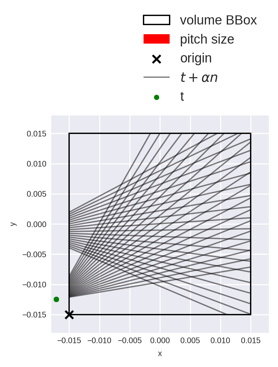
In the 2D case, the parametrization is best explained by the figure below:

2D Imaging#
Let’s try to reconstruct a phantom using different scanning geometries, each having the same number of total rays cast into the medium:
2D parallel beam with equi-spaced offsets.
2D fan beam.
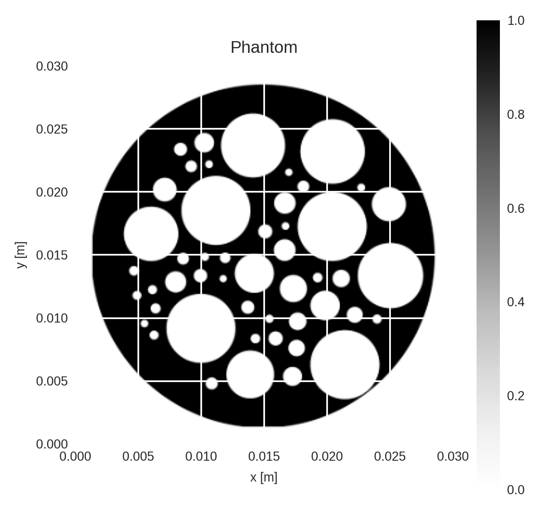
We will use the phantom below for all experiments.
[2]:
def create_2D_phantom(shape: tuple[int], seed: int) -> np.ndarray:
    # in: (N_h, N_w) phantom dimensions [px]
    # out: (N_h, N_w) phantom
    import xdesign as xd

    np.random.seed(seed)
    substrate = xd.Foam(size_range=[0.1, 0.01], gap=0.025, porosity=0.5)
    I = xd.discrete_phantom(substrate, np.mean(shape, dtype=int))  # produce image at average resolution
    I = np.pad(I, int(0.05 * I.shape[0]))  # 5% axial pad

    I = ski.transform.rescale(I, scale=np.array(shape) / I.shape[0])  # rescale to user dimensions
    I = (I - I.min()) / I.ptp()
    return I

N_side = 300  # N_px = N_side**2
pitch = 1e-4  # m/px [can differ per axis]
phantom = create_2D_phantom(shape=(N_side, N_side), seed=5)
im_kwargs = dict(
    origin="lower",
    extent=[0, N_side * pitch, 0, N_side * pitch],
)

fig, ax = plt.subplots()
im = ax.imshow(phantom, **im_kwargs)
fig.colorbar(im)
ax.set_xlabel("x [m]")
ax.set_ylabel("y [m]")
ax.set_title("Phantom")
[2]:
Text(0.5, 1.0, 'Phantom')
Parallel Beam: Uniform Offsets#
Let’s first look at a baseline setup similar to what scikit-image’s radon()🔗 and iradon()🔗 functions would produce: a parallel-beam scan with equi-spaced lines and uniformly-distributed scan directions.
[3]:
N_angle = 100
N_offset = 200

# Let's build the necessary components to instantiate the operator. ========================
angle = np.linspace(0, np.pi, N_angle, endpoint=False)
n = np.stack([np.cos(angle), np.sin(angle)], axis=1)

t = n[:, [1, 0]] * np.r_[-1, 1]  # <n, t> = 0
t_max = pitch * N_side / 2 * 1.1  # 10% over ball radius
t_offset = np.linspace(-t_max, t_max, N_offset, endpoint=True)

n_spec = np.broadcast_to(n.reshape(N_angle, 1, 2), (N_angle, N_offset, 2))  # (N_angle, N_offset, 2)
t_spec = t.reshape(N_angle, 1, 2) * t_offset.reshape(N_offset, 1)  # (N_angle, N_offset, 2)
t_spec += pitch * N_side / 2  # Move anchor point to the center of volume.
# ==========================================================================================

op_para_u = pxo.RayXRT(
    dim_shape=(N_side, N_side),
    origin=0,  # bottom-left corner of volume located at (0, 0)
    pitch=pitch,  # pixel dimensions. (Can vary per axis.)
    n_spec=n_spec.reshape(-1, 2),  # (N_ray, 2) directions
    t_spec=t_spec.reshape(-1, 2),  # (N_ray, 2)
)
It can be tricky to correctly parametrize the rays. The diagnostic_plot() method can be used to verify everything is correct. By default diagnostic_plot() shows all rays going through the volume. For visualization purposes, let’s only plot every \(N\)-th angle and \(K\)-th offset.
[4]:
N, K = 10, 20
ray_idx = np.arange(N_angle * N_offset).reshape(N_angle, N_offset)[::N,::K]

fig = op_para_u.diagnostic_plot(ray_idx)
fig.show()
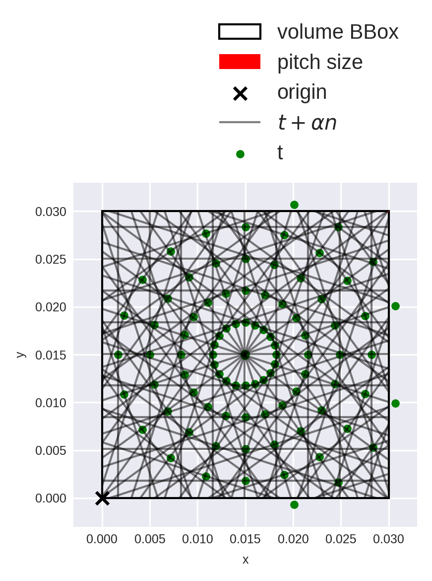
The construction seems ok for a parallel-beam scan: angles/offsets are distributed uniformily, and we can already see that the lines concentrate in the center of the volume. (More on this later.)
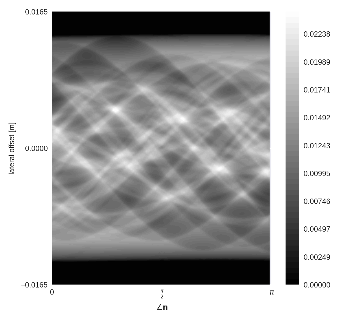
Now that we created the XRay operator, let’s compute the sinogram and visualize it.
[5]:
# Compute sinogram
sinogram = op_para_u.apply(phantom).reshape(N_angle, N_offset)  # (N_angle, N_offset)


# And plot it
N_level = 50
fig, ax = plt.subplots()
ANGLE, OFFSET = np.meshgrid(angle, t_offset, indexing="ij")
contour = ax.contourf(
    ANGLE,
    OFFSET,
    sinogram,
    levels=np.linspace(0, sinogram.max(), N_level),
    cmap='grey',
)
cbar = fig.colorbar(contour, ax=ax)
ax.set_xlabel(r"$\angle \mathbf{n}$")
ax.set_xticks(
    ticks=[0, np.pi/2, np.pi],
    labels=["0", r"$\frac{\pi}{2}$", r"$\pi$"],
)
ax.set_ylabel(r"lateral offset [m]")
ax.set_yticks(
    ticks=[t_offset.min(), 0, t_offset.max()],
    labels=None,
);
Now that we have the sinogram, let’s invert the imaging process to (try to) reconstruct an image which produced it. We will try 2 methods:
Plain back-projection of the sinogram data into the image domain.
Forming the least-squares image. The conventional Filtered-BackProjection algorithm (FBP) should produce similar images, but let’s stick to an undampened CG method to compute the pseudo-inverse for simplicity.
[6]:
# Compute backprojected image and LSQ image. =======================
I_BP = op_para_u.adjoint(sinogram.reshape(-1))
I_LSQ = op_para_u.pinv(sinogram.reshape(-1), damp=0)

# Plot the images ==================================================
fig, ax = plt.subplots(1, 3, figsize=[4, 6])
ax[0].imshow(phantom, **im_kwargs)
ax[1].imshow(I_BP, **im_kwargs)
ax[2].imshow(I_LSQ, **im_kwargs)
ax[0].set_title("Ground-Truth")
ax[1].set_title("BackProj")
ax[2].set_title("LS")
for _ax in ax:
    _ax.axis("off")

# aliases to compare against fan-beam later on.
I_BP_u = I_BP
I_LSQ_u = I_LSQ
INFO:/tmp/pyxu_4xlaowpq:[2024-04-22 15:33:54.750346] Iteration 0
        iteration: 0
        AbsError[residual]: 0.021843749200722698
        N_iter: 1.0
INFO:/tmp/pyxu_4xlaowpq:[2024-04-22 15:33:54.873656] Iteration 1
        iteration: 1
        AbsError[residual]: 0.0018200192757085538
        N_iter: 2.0
INFO:/tmp/pyxu_4xlaowpq:[2024-04-22 15:33:55.001849] Iteration 2
        iteration: 2
        AbsError[residual]: 0.0012724930894719814
        N_iter: 3.0
INFO:/tmp/pyxu_4xlaowpq:[2024-04-22 15:33:55.122514] Iteration 3
        iteration: 3
        AbsError[residual]: 0.0005394651661135211
        N_iter: 4.0
INFO:/tmp/pyxu_4xlaowpq:[2024-04-22 15:33:55.248853] Iteration 4
        iteration: 4
        AbsError[residual]: 0.00029948792312451593
        N_iter: 5.0
INFO:/tmp/pyxu_4xlaowpq:[2024-04-22 15:33:55.471487] Iteration 5
        iteration: 5
        AbsError[residual]: 0.0001959775032532727
        N_iter: 6.0
INFO:/tmp/pyxu_4xlaowpq:[2024-04-22 15:33:55.594374] Iteration 6
        iteration: 6
        AbsError[residual]: 0.00010660540950964133
        N_iter: 7.0
INFO:/tmp/pyxu_4xlaowpq:[2024-04-22 15:33:55.721348] Iteration 7
        iteration: 7
        AbsError[residual]: 7.813945938822347e-05
        N_iter: 8.0
INFO:/tmp/pyxu_4xlaowpq:[2024-04-22 15:33:55.722198] Stopping Criterion satisfied -> END
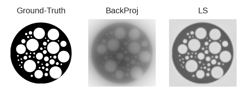
Some high-level remarks just by looking at these images:
The backprojected image has low contrast.
The least-squares image allows us to identify the porous structure more easily.
Fan Beam#
Sometimes parallel-beam is not possible due to application requirements such as fast(er) scanning. Fan beam is therefore an interesting scan geometry in practice.
We will take the same \(N_{\mathrm{angle}}\) and \(N_{\mathrm{offset}}\) settings as in parallel beam, but where \(N_{\mathrm{angle}}\) refers to the number of “emitter” locations, and \(N_{\mathrm{offset}}\) now corresponds to the number of detectors spread along the edge of the image.
[7]:
# In the parallel-beam setups above, we had fixed `origin=0` and shifted `t_spec` to be centered at the volume
# mid-point, i.e. (N_side * pitch / 2). For fan-beam, it is easier to center the volume at the origin of the reference
# system, i.e. `origin = -(N_side * pitch / 2)`, and define `n/t_spec` for one source position. Subsequent src/detector
# positions are then obtained by applying a rotation matrix.

# Let's build the necessary components to instantiate the operator. ========================
radius = (N_side * pitch / np.sqrt(2))  # be at diagonal distance
tx = np.r_[-1, 0] * radius  # (2,)
t_max = N_side * pitch / np.sqrt(2)
t_offset = np.linspace(-t_max, t_max, N_offset, endpoint=True)
rx = np.stack([radius * np.ones(N_offset), t_offset], axis=-1)  # (N_offset, 2)

t = np.broadcast_to(tx, (N_offset, 2))
n = rx - tx  # vectors pointing from unique TX to all RX.

angle = np.linspace(0, 2 * np.pi, N_angle, endpoint=False)
R = np.zeros((N_angle, 2, 2))
R[:, 0, 0] = R[:, 1, 1] = np.cos(angle)
R[:, 1, 0] = np.sin(angle)
R[:, 0, 1] = -np.sin(angle)

n_spec = (R @ n.T).transpose(0, 2, 1)  # (N_angle, N_offset, 2)
t_spec = (R @ t.T).transpose(0, 2, 1)  # (N_angle, N_offset, 2)
# ==========================================================================================


op_fan = pxo.RayXRT(
    dim_shape=(N_side, N_side),
    origin=-N_side * pitch / 2,  # center of volume located at (0, 0)
    pitch=pitch,  # pixel dimensions. (Can vary per axis.)
    n_spec=n_spec.reshape(-1, 2),  # (N_ray, 2) directions
    t_spec=t_spec.reshape(-1, 2),  # (N_ray, 2)
)
Let’s again verify that the rays are instantiated correctly. We’ll limit the visualization to 2 “emitters”, and sub-sample the outgoing beam-count for visualization purposes:
[8]:
ray_idx = np.arange(N_angle * N_offset).reshape(N_angle, N_offset)[[1, 10], ::10]

fig = op_fan.diagnostic_plot(ray_idx)
fig.show()
We can already see an interesting difference with respect to parallel-beam setups: the ray density is higher in the periphery than in the center region.
Plotting the sinogram is more complex than in the parallel-beam case, so let’s skip that step and instead see what the back-projected and least-squares images look like.
[9]:
# Compute backprojected image and LSQ image. =======================
sinogram = op_fan.apply(phantom).reshape(N_angle, N_offset)
I_BP = op_fan.adjoint(sinogram.reshape(-1))
I_LSQ = op_fan.pinv(sinogram.reshape(-1), damp=0)

# Plot the images ==================================================
fig, ax = plt.subplots(1, 5, figsize=[5, 7])
ax[0].imshow(phantom, **im_kwargs)
ax[1].imshow(I_BP, **im_kwargs)
ax[2].imshow(I_LSQ, **im_kwargs)
ax[3].imshow(I_BP_u, **im_kwargs)
ax[4].imshow(I_LSQ_u, **im_kwargs)
ax[0].set_title("Ground-Truth")
ax[1].set_title("BP (Fan)")
ax[2].set_title("LSQ (Fan)")
ax[3].set_title("BP (Par)")
ax[4].set_title("LSQ (Par)")
for _ax in ax:
    _ax.axis("off")
INFO:/tmp/pyxu_tm_ea5j5:[2024-04-22 15:33:56.745022] Iteration 0
        iteration: 0
        AbsError[residual]: 0.030986974144406307
        N_iter: 1.0
INFO:/tmp/pyxu_tm_ea5j5:[2024-04-22 15:33:56.893634] Iteration 1
        iteration: 1
        AbsError[residual]: 0.0017455433116292133
        N_iter: 2.0
INFO:/tmp/pyxu_tm_ea5j5:[2024-04-22 15:33:57.043016] Iteration 2
        iteration: 2
        AbsError[residual]: 0.0012417042429075098
        N_iter: 3.0
INFO:/tmp/pyxu_tm_ea5j5:[2024-04-22 15:33:57.186023] Iteration 3
        iteration: 3
        AbsError[residual]: 0.0004833370042454062
        N_iter: 4.0
INFO:/tmp/pyxu_tm_ea5j5:[2024-04-22 15:33:57.327290] Iteration 4
        iteration: 4
        AbsError[residual]: 0.00026830554970115237
        N_iter: 5.0
INFO:/tmp/pyxu_tm_ea5j5:[2024-04-22 15:33:57.472082] Iteration 5
        iteration: 5
        AbsError[residual]: 0.00016592683028195928
        N_iter: 6.0
INFO:/tmp/pyxu_tm_ea5j5:[2024-04-22 15:33:57.619500] Iteration 6
        iteration: 6
        AbsError[residual]: 9.948386938706681e-05
        N_iter: 7.0
INFO:/tmp/pyxu_tm_ea5j5:[2024-04-22 15:33:57.620385] Stopping Criterion satisfied -> END
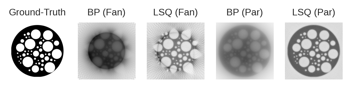
Based on the plots, we can already see some interesting behaviour:
Fan-beam can only image accurately the circular region seen by all fans. Parallel-beam in contrast can see uniformly-well everywhere.
Fan-beam images have lower contrast compared to parallel beam setups.
A finer analysis is of course possible, but we hope to have shown how the scanning geometry impacts image reconstruction. The versatile RayXRT() class is therefore a handy tool in the computational scientist’s toolbox!
(Also note that weighted XRTs are also supported.)